Lec 8: Level curves; partial derivatives; tangent plane | MIT 18.02 Multivariable Calculus, Fall 07

The paragraph introduces the transition from studying geometry in space to delving into calculus, specifically focusing on functions of several variables. It emphasizes the shift from single-variable functions, exemplified by a sine function, to multi-variable functions where the value is determined by multiple parameters, such as x and y. The paragraph also touches on the concept of domain of definition and provides real-world examples, like temperature as a function of geographical coordinates and elevation, to illustrate the application of multi-variable functions.

This section discusses the challenges and methods of visualizing functions of two variables. It explains that while simple functions can be represented as planes in three-dimensional space, more complex functions require different approaches. The paragraph introduces the concept of graphing functions like z = f(x, y) to represent surfaces in space and uses the function f(x, y) = -y as an example to illustrate how a function's graph can be a plane. It also mentions the difficulty in graphing functions with more than two variables and the tools that remain consistent regardless of the number of variables involved.

The paragraph delves into the process of visualizing functions of two variables through graphs and contour plots. It explains how to sketch the graph of a function by considering the function's value at various points in the x, y plane and then plotting these points in three-dimensional space to form a surface. The paragraph uses the function f(x, y) = 1 - x^2 - y^2 as an example to demonstrate how to visualize the surface by examining cross-sections in different planes and understanding the function's behavior at the x, y plane. It also highlights the utility of computer-generated graphs for more complex functions.

This section introduces contour plots as an alternative method for representing functions of two variables on a two-dimensional surface. It compares contour plots to geographical maps, where lines represent constant elevations or values of the function. The paragraph explains that contour plots consist of lines connecting points of equal function value and that these plots can quickly convey the value of the function at a given point. It also describes how to interpret the spacing of contour lines to determine the steepness of the function's surface.

The paragraph provides real-world examples of contour plots, such as topographical maps and temperature maps, to illustrate their practical applications. It explains how topographical maps show altitude levels and how temperature maps use color-coded contour lines to represent temperature variations. The section emphasizes the importance of becoming familiar with contour plots for understanding functions of two variables and their visualization.

This section discusses how contour plots can be used to analyze the behavior of functions of two variables. It explains that by observing the spacing and arrangement of contour lines, one can infer the rate of change and the direction of increase or decrease in the function's value. The paragraph also demonstrates how to calculate level curves for given function values and how the distance between contour lines indicates the steepness of the function, with closer lines signifying steeper gradients.

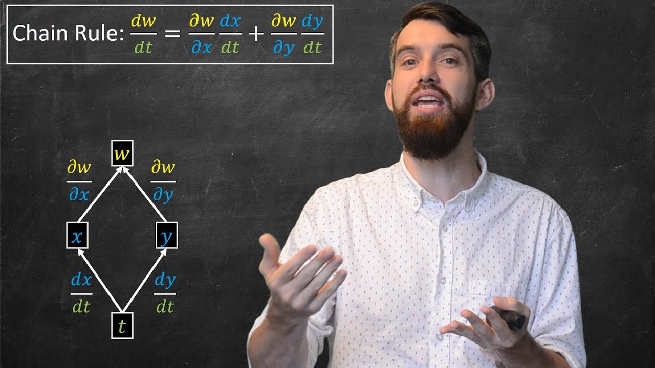
The paragraph introduces the concept of derivatives in the context of functions of one variable before transitioning to partial derivatives for functions of two variables. It explains that partial derivatives involve differentiating with respect to one variable while treating the others as constants. The section provides a geometric interpretation of partial derivatives as the slope of a tangent line to the graph of a function in a plane parallel to either the x or y axis. It also outlines the notation used for partial derivatives and emphasizes their importance in understanding the rate of change of multi-variable functions.

This final paragraph focuses on the computation of partial derivatives, highlighting the process as similar to that of single-variable derivatives but with the key difference of treating one variable as constant while differentiating with respect to another. The paragraph provides an example calculation of partial derivatives for the function f(x, y) = x^3y^2, demonstrating how to treat y as a constant when differentiating with respect to x, and vice versa. It concludes with a note on the simplicity of partial derivative computation once the variable and constant roles are clear.