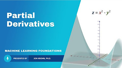
Math 11 - Sections 6.1- 6.2
TLDRThe video script is a comprehensive lecture on multivariate calculus, focusing on functions of several variables and their derivatives. It begins by contrasting single-variable functions, such as y = x^2 - 9x + 2, with multivariate functions, which depend on more than one independent variable, exemplified by a student's test score being influenced by homework completion and study hours. The lecture introduces notation for functions of multiple variables, such as f(x, y), and discusses evaluating these functions at given points, as demonstrated with the function f(x, y) = y^2 + 2xy. The crux of the script delves into partial derivatives, illustrating how to treat one variable as constant while differentiating with respect to another. This concept is applied to various functions, including those with multiple variables and constants. The lecture also covers second-order partial derivatives and their implications, emphasizing the need for consistency in results when deriving in different orders. Practical applications, such as the Cobb-Douglas production function in economics, highlight the significance of marginal productivities in decision-making. The script concludes with an interactive approach, encouraging students to solve problems and verify their understanding through practice.
Takeaways
- 📚 The lecture covers two sections: 6.1 on functions of several variables, and 6.2 on derivatives of such functions, with a focus on partial derivatives.
- 🔢 Functions can depend on more than one variable, which is a shift from the single-variable functions previously discussed.
- 📈 The concept of treating one variable as constant while differentiating with respect to another is a key idea in understanding partial derivatives.
- 🎓 Examples are provided to illustrate how to calculate function values at given points and how to work with different notations such as Newton's and Leibniz's notation.
- 🤔 The importance of understanding that constant multiples do not go to zero when taking derivatives is emphasized, which can be a common source of confusion.
- 📊 The application of partial derivatives is demonstrated through the Cobb-Douglas production function model, which is used to determine marginal productivities in economics.
- 🧮 Calculating second-order partial derivatives is shown to be a straightforward extension of first-order partial derivatives, with the added complexity of multiple differentiation steps.
- 🤓 The use of parentheses and the order of operations in calculations is highlighted as crucial for accuracy, especially when dealing with powers and division.
- 📉 The economic application of the Cobb-Douglas model helps in decision-making regarding the allocation of resources between labor and capital for production.
- 💡 The marginal productivity of labor and capital is calculated to determine the additional units produced by adding one more unit of either labor or capital.
- 📚 Students are encouraged to practice problems from both Chapter 3 and Chapter 6, as both will be covered in the upcoming exam.
Q & A
What are the two sections being discussed in the transcript?
-The two sections being discussed are 6.1 and 6.2, which cover functions of several variables and derivatives of functions of several variables, respectively.
What is the difference between a function of one variable and a function of several variables?
-A function of one variable, such as y = x^2 - 9x + 2, has a single independent variable (x), whereas a function of several variables depends on more than one independent variable, which can affect the outcome of the function.
How is the notation for functions of several variables typically written?
-Functions of several variables can be written using Newton's notation as f(x, y) or in Leibnitz notation as z = 3x - 9y^2, where x and y are independent variables and z is the dependent variable.
What is a partial derivative?
-A partial derivative is a derivative that takes the rate of change of one variable at a time, treating the other variables as constants.
How does the process of taking partial derivatives relate to the concept of slopes in a three-dimensional space?
-Taking partial derivatives is akin to finding the slope of a function at a particular point in a three-dimensional space. It shows how the function changes with respect to one variable while holding the other variables constant.
What is the Cobb-Douglas model mentioned in the transcript?
-The Cobb-Douglas model is a production function used in economics that represents the relationship between the quantity of output produced and the quantities of various inputs used. It is given by the formula P = A * X^(α) * Y^(β), where P is the production, X and Y are inputs, and α and β are constants that sum up to 1.
What are marginal productivities in the context of the Cobb-Douglas model?
-Marginal productivities in the context of the Cobb-Douglas model refer to the partial derivatives of the production function with respect to the inputs (labor and capital). They indicate the additional output that can be produced by adding one more unit of an input while holding the other input constant.
How does the transcript demonstrate the calculation of the marginal productivity of labor and capital?
-The transcript demonstrates the calculation by evaluating the partial derivatives of the Cobb-Douglas production function at specific levels of labor (X) and capital (Y). It shows that by adding one unit of labor, 7,680 more units are produced, while adding one unit of capital results in 360 more units.
What is the significance of finding the second-order partial derivatives in the transcript?
-Second-order partial derivatives provide information about the curvature of the function. In the context of the Cobb-Douglas model, they can be used to analyze the elasticity of the production function with respect to changes in inputs.
How does the transcript address the potential confusion between constant multiples and variables when taking derivatives?
-The transcript clarifies that constant multiples do not go to zero when taking derivatives if they are part of a product with a variable. It emphasizes the importance of understanding whether a term is a constant or a variable when applying the rules of differentiation.
What is the recommendation for students when practicing taking partial derivatives?
-The recommendation is to practice by pausing the video, working through the problem, and then resuming the video to compare answers. This helps in understanding the process and identifying any mistakes made during the calculation.
Outlines
📚 Introduction to Functions of Several Variables
The video begins with an introduction to functions involving multiple variables, contrasting them with single-variable functions. It explains that functions like Y = X^2 - 9X + 2 have one independent variable, X, whereas functions in several variables, such as F(X, Y), depend on more than one variable, like the number of homework problems done and hours studied affecting a student's test score. The notation for such functions is also discussed, including Newton's and Leibniz's notations, with examples provided to illustrate their use.
🔍 Evaluating Function Values at Specific Points
The script continues with an example of evaluating function values at specific points, such as F(-2, 0) and F(3, 2), using the given function F(X, Y) = Y^2 + 2XY + X^3. The process involves substituting the given X and Y values into the function and performing the necessary calculations, resulting in the function's value at those points, which are then interpreted in a three-dimensional context.
📈 Application: Calculating Stock Yield
An application of functions of several variables is demonstrated through the example of calculating the yield of a stock, which is a function of both the dividend and the stock's price. The formula for yield is given as Y = D/P, where D is the dividend and P is the price. Using historical data for the Texas Instrument stock price and dividend, the script shows how to calculate the yield on April 1st, 2014.
🧮 Understanding Partial Derivatives
The concept of partial derivatives is introduced, emphasizing that they involve differentiating with respect to one variable while keeping the other variables constant. The script explains the notation and calculation process for partial derivatives, using a simple function f(X, Y) = 3X + 5Y to illustrate. It also discusses the importance of treating the other variables as constants when taking partial derivatives.
📈 Calculating Partial Derivatives and Their Values at Points
The script delves into calculating partial derivatives of more complex functions, such as Z = 2X^3 + 3XY - X, and evaluating these derivatives at specific points, like the partial of Z with respect to X at (-2/3, -3) and the partial of Z with respect to Y at (0, -5). The process involves applying the rules of differentiation to each term of the function, considering the other variable as constant.
🧐 Challenging Partial Derivatives with Logarithms and Exponents
The video tackles more complex scenarios involving partial derivatives, including functions with logarithms and exponents such as f(X, Y) = Y * ln(X) + 2Y. The script outlines the steps for finding partial derivatives with respect to both X and Y, emphasizing the use of the chain rule and product rule where applicable. It also encourages students to practice and review previous problems to solidify their understanding.
🔢 Second-Order Partial Derivatives and Their Applications
The script introduces second-order partial derivatives, which are the partial derivatives of first-order partial derivatives. It explains the four different types of second-order partial derivatives and emphasizes that the order of differentiation does not matter for certain pairs, resulting in equal values. Examples are provided to illustrate the calculation of these derivatives, and the script advises students to verify their work by comparing the results of different orders of differentiation.
🏭 Applying Partial Derivatives to the Cobb-Douglas Production Function
An application of second-order partial derivatives is shown using the Cobb-Douglas production function, which is used to determine the marginal productivities of labor and capital. The script calculates the production units based on given labor and capital units and then finds the partial derivatives with respect to both labor (X) and capital (Y). These derivatives are evaluated at specific points to determine the additional units produced by adding one unit of labor or capital, providing insight into the most efficient way to increase production.
📝 Wrapping Up the Lesson
The video concludes with a reminder for students to practice the material, especially the calculations of partial derivatives, as it will be part of the upcoming test. The instructor encourages students to complete their homework and to ask any questions they may have during the live session. The emphasis is on understanding the process of taking derivatives in functions of several variables and applying them to real-world scenarios.
Mindmap
Keywords
💡Function of Several Variables
💡Partial Derivative
💡Newton's Notation
💡Leibniz Notation
💡Cobb-Douglas Model
💡Marginal Productivity
💡Second-Order Partial Derivatives
💡Constant Multiple Rule
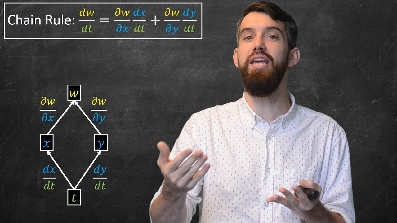
💡Chain Rule
💡Product Rule
💡Independent and Dependent Variables
Highlights
Introduction to functions of several variables, emphasizing their dependence on more than one independent variable.
Explanation of how the performance on a test can be a function of multiple factors, such as homework completion and study hours.
Discussion on the stock market as an example of a function influenced by various variables like consumer sentiment and interest rates.
Illustration of different notations for functions of several variables, such as f(X, Y) and Z = 3X - 9Y^2.
Calculation of function values for given variable values, demonstrated through examples from a textbook.
Introduction to partial derivatives, highlighting their role in determining the rate of change of a function with respect to one variable while holding others constant.
Use of Newton's notation and Leibnitz notation in expressing derivatives and partial derivatives.
Application of partial derivatives in economics, specifically in the Cobb-Douglas production function model.
Calculation of marginal productivities to determine the additional output from one more unit of labor or capital.
Practical application of the Cobb-Douglas model to decide between hiring more labor or investing in more capital based on cost-effectiveness.
Emphasis on the importance of treating non-variable terms as constants when taking partial derivatives.
Demonstration of how to calculate second-order partial derivatives and the significance of their order.
Explanation of the product rule and chain rule in the context of taking partial derivatives.
Use of t-charts for visualizing the impact of changing one variable on the function while keeping the other constant.
Guidance on practicing problems by pausing the video and working through them independently to check understanding.
Clarification on the concept of slopes in the context of three-dimensional space and how partial derivatives relate to them.
Advice on checking one's work by comparing the results of different orders of partial derivatives to ensure accuracy.
Transcripts
Browse More Related Video


5.0 / 5 (0 votes)
Thanks for rating: