Lagrange multipliers, using tangency to solve constrained optimization
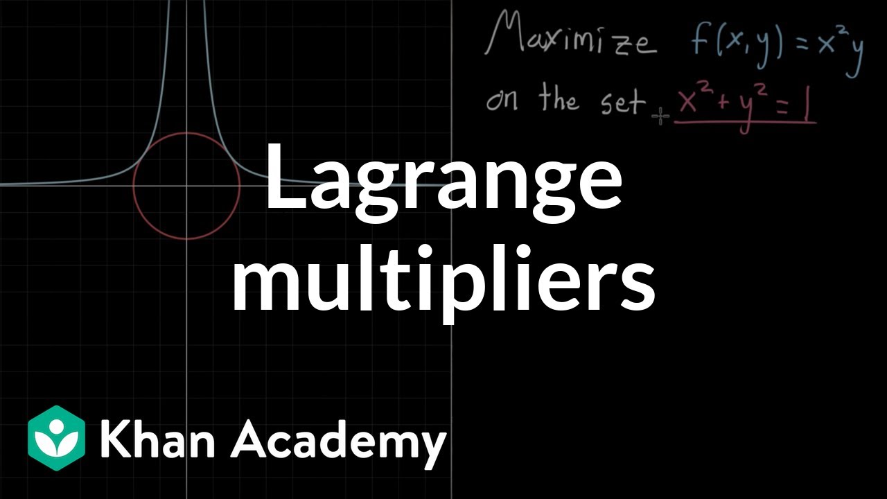
TLDRThis educational video delves into solving a constrained optimization problem, where the objective is to maximize the function f(x, y) = x^2 * y under the constraint x^2 + y^2 = 1. The instructor visualizes the problem using contour lines and introduces the concept of a gradient to find the maximum value without exceeding the constraint. The key is to identify the point of tangency between the contour lines of the function and the constraint, using the gradient vectors. The video also explains the use of the Lagrange multiplier, a technique to solve constrained optimization problems, setting the stage for solving the equations in the next video.
Takeaways
- 📚 The video introduces a constrained optimization problem where the goal is to maximize the function f(x, y) = x^2 * y subject to the constraint x^2 + y^2 = 1.
- 📈 The constraint is visualized as a unit circle on the x, y plane, with the function's contour lines representing different constant values of f(x, y).
- 🔍 To maximize the function, one must increase the value of the constant c in the contour lines without the point falling off the circle, which occurs at the point of tangency.
- 📐 The concept of tangency is crucial, as the point of maximization is where the contour line of f(x, y) is tangent to the constraint circle.
- 🛠 The gradient is the main tool used to solve the problem, with the gradient vectors being perpendicular to the contour lines at every point they intersect.
- 🔄 The gradient of the function f and the constraint function g (x^2 + y^2) are used to find the point of tangency, with the gradient of f being proportional to the gradient of g.
- 🔢 The proportionality between the gradients is expressed using a Lagrange multiplier, λ, which is a scalar that relates the gradients of the two functions at the point of maximization.
- 🔄 The gradients of f and g are vectors with components derived from the partial derivatives of the respective functions with respect to x and y.
- 🧩 The system of equations to solve the optimization problem includes the proportionality of the gradients (two separate equations) and the original constraint equation.
- 🔑 The Lagrange multiplier, λ, is not just a variable but has a deeper meaning in physical contexts and represents a balance between the rate of change of the objective function and the constraint.
- 📝 The next steps involve solving the system of equations algebraically to find the values of x, y, and λ that maximize the function subject to the constraint.
Q & A
What is the function being maximized in the video script?
-The function being maximized is f(x, y) = x^2 * y, subject to the constraint x^2 + y^2 = 1.
What is the geometric interpretation of the constraint x^2 + y^2 = 1 in the context of the problem?
-The constraint x^2 + y^2 = 1 represents a unit circle in the x, y plane, where all points on the circle satisfy the constraint.
What is the significance of the contour lines in the video script?
-Contour lines represent sets of points where the function f(x, y) has a constant value. They help visualize the levels of the function and are used to find the maximum value subject to the given constraint.
Why is the gradient vector important in solving this optimization problem?
-The gradient vector is important because it points in the direction of the steepest ascent of the function. In the context of constrained optimization, it helps identify the point of tangency between the contour lines of the objective function and the constraint.
What does it mean for the contour lines of f(x, y) and g(x, y) to be tangent to each other?
-For the contour lines to be tangent to each other means that at the point of tangency, the gradient vectors of both functions are perpendicular to the contour lines and proportional to each other, indicating the maximum or minimum of the function subject to the constraint.
What is the role of the Lagrange multiplier in this optimization problem?
-The Lagrange multiplier, denoted by lambda (λ), is a scalar that ensures the proportionality between the gradient of the objective function f and the gradient of the constraint function g at the point of tangency.
How many equations are needed to solve for the unknowns x, y, and the Lagrange multiplier λ?
-Three equations are needed to solve for the unknowns x, y, and λ. These include the two proportionality equations derived from the gradients and the original constraint equation x^2 + y^2 = 1.
What is the gradient of the function g(x, y) = x^2 + y^2?
-The gradient of g is a vector with components ∂g/∂x = 2x and ∂g/∂y = 2y, which simplifies to the vector <2x, 2y>.
How are the partial derivatives of f(x, y) = x^2 * y calculated?
-The partial derivative with respect to x is ∂f/∂x = 2xy, treating y as a constant, and with respect to y is ∂f/∂y = x^2, treating x as a constant.
What is the relationship between the gradients of f and g at the point of maximum?
-At the point of maximum, the gradient of f is proportional to the gradient of g, with the proportionality constant being the Lagrange multiplier λ. This means that the gradients are parallel and have the same direction.
What does the instructor suggest for further understanding of the relationship between the gradient and contour lines?
-The instructor suggests watching another video that explains the relationship between the gradient and contour lines in more detail, as it is crucial for understanding the optimization process.
Outlines
📚 Introduction to Constrained Optimization
The instructor begins by revisiting a constrained optimization problem introduced in a previous video. The goal is to maximize the function f(x, y) = x^2 * y, subject to the constraint x^2 + y^2 = 1, which is visualized as a circle on the x, y plane. The function's contours are depicted as curvy lines representing constant values of f(x, y), with higher values of c resulting in contours closer to the circle's edge. The maximization strategy involves increasing the constant c without the contour line falling off the circle, ideally at the point of tangency between the contour and the circle. The instructor emphasizes the importance of the gradient in solving this problem and introduces the concept of the gradient field for function f. The relationship between the gradient and contour lines is explained, highlighting that the gradient vectors are perpendicular to the contour lines at every point of intersection. The video concludes with the introduction of the constraint function g(x, y) = x^2 + y^2 and its gradient, setting the stage for the use of the Lagrange multiplier technique in the next part of the explanation.
🔍 Applying the Gradient and Lagrange Multiplier
The second paragraph delves into the application of the gradient in solving the constrained optimization problem. The instructor calculates the gradients of both functions f and g, highlighting that they are vectors composed of partial derivatives. The gradient of g is found to be <2x, 2y>, while the gradient of f is <2xy, x^2>. Using the concept of the Lagrange multiplier, denoted by λ, the gradients of f and g are set proportional to each other, resulting in two equations that relate x, y, and λ. The instructor points out that these two equations, along with the original constraint x^2 + y^2 = 1, form a system of three equations with three unknowns. This system is necessary to solve for the values of x, y, and λ that maximize the function f under the given constraint. The instructor also mentions that λ is not merely a variable but has a significant physical interpretation in practical optimization problems. The summary ends with a preview of the next video, where the algebraic solution to the system will be discussed, as well as the interpretation of the Lagrange multiplier.
Mindmap
Keywords
💡Constrained Optimization
💡Function f(x, y)
💡Constraint
💡Contour Lines
💡Gradient
💡Tangency
💡Lagrange Multiplier
💡Gradient of g
💡Partial Derivatives
💡Proportionality
💡Algebraic Solution
Highlights
Introduction to a constrained optimization problem with a specific function to maximize and a constraint.
Visualization of the problem on the x, y plane with a circle representing the constraint and contour lines for the function.
Explanation of how to maximize the function by increasing the value of a constant without falling off the circle, with tangency being key.
Use of the gradient as the main tool for solving the optimization problem.
Illustration of the relationship between the gradient and contour lines, showing that gradient vectors are perpendicular to contour lines.
Identification of the point of tangency where the gradient of the function is perpendicular to both curves.
Introduction of the function g(x, y) to represent the constraint and its contour lines.
Discussion on the gradient of g and its perpendicularity to the contour lines of g.
Introduction of the Lagrange multiplier, a key concept in solving constrained optimization problems.
Explanation of the proportionality between the gradients of f and g at the point of tangency, using the Lagrange multiplier.
Derivation of the gradient vectors for both f and g, and setting up the proportionality equations.
Transformation of the vector equation into two separate scalar equations involving the Lagrange multiplier.
Introduction of the constraint equation as the third necessary equation to solve for x, y, and the Lagrange multiplier.
Emphasis on the importance of the constraint equation in characterizing the optimization problem.
Promise of solving the equations algebraically in the next video and discussing the encapsulation of the equations.
Teaser about the interpretation of the Lagrange multiplier in physical contexts and its significance beyond the mathematical solution.
Transcripts
Browse More Related Video


5.0 / 5 (0 votes)
Thanks for rating: