Finishing the intro lagrange multiplier example
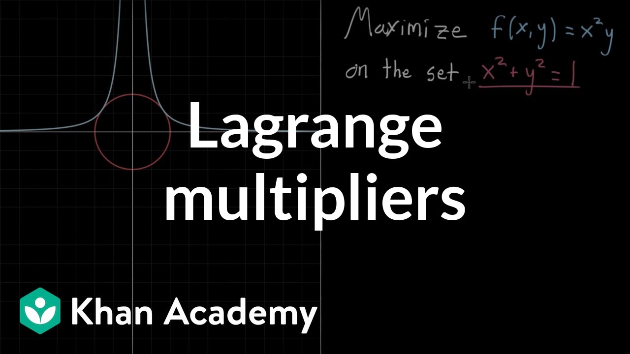
TLDRThis video script delves into solving a constrained optimization problem using the Lagrange Multiplier technique. The instructor guides through the process of maximizing a function subject to the constraint x^2 + y^2 = 1. By simplifying and solving a system of equations, the script identifies potential solutions, excluding the case where x = 0. It highlights the importance of checking for such special cases. The script concludes by evaluating the function at the possible solutions, determining the maximum value and emphasizing the technique's significance over specific algebraic details.
Takeaways
- 📚 The video discusses a constrained optimization problem involving maximizing a function subject to the constraint x^2 + y^2 = 1.
- 🔍 Geometric reasoning is used to simplify the problem into a system of equations that need to be solved.
- ✂️ An assumption is made that x is not zero to cancel out terms, with a note to revisit the possibility of x being zero later.
- 📉 The instructor simplifies the equations step by step, eventually finding that y = λ and x^2 = 2y^2.
- 🔢 Solving for y leads to y being plus or minus the square root of one third, and subsequently, x is found to be plus or minus the square root of two thirds.
- 📌 Four potential solutions for x and y are identified, considering both positive and negative square roots.
- 🚫 The possibility of x being zero is explored and dismissed since it would not satisfy the constraint x^2 + y^2 = 1.
- 🔍 The Lagrange Multiplier technique is emphasized as the key method for finding points of tangency between contour lines.
- 📝 The function to be maximized is f(x, y) = x^2 * y, and the values of x and y from the potential solutions are substituted into this function.
- 📊 It's noted that negative values for y would result in a negative function value, so only positive combinations are considered for the maximum.
- 🏁 The final maximum value of the function is found to be two thirds times the square root of one third, with two different maximizing points.
- 💡 The importance of checking work and understanding the process, rather than just the algebraic result, is highlighted as the main takeaway.
Q & A
What is the main topic discussed in the video script?
-The main topic discussed in the video script is the application of the Lagrange Multiplier technique to solve a constrained optimization problem involving a function to be maximized on a set defined by x squared plus y squared equals one.
What is the constraint set in the optimization problem presented in the script?
-The constraint set in the optimization problem is the set of all points (x, y) where x squared plus y squared equals one, which is the equation of a circle with radius one centered at the origin.
What does the instructor initially assume about the variable x in the system of equations?
-The instructor initially assumes that x is not equal to zero in order to cancel out the x terms in the system of equations.
What is the simplified form of the equation that results from assuming x is not zero?
-The simplified form of the equation that results from this assumption is y equals lambda, where lambda represents the Lagrange Multiplier.
How does the instructor use the simplified equation to solve for x squared?
-The instructor uses the simplified equation (y equals lambda) to replace lambda in the equation x squared equals lambda times two times y, resulting in x squared equals two times y squared.
What is the result of substituting x squared with two times y squared in the equation?
-Substituting x squared with two times y squared in the equation simplifies it to three times y squared equals one, which further simplifies to y squared equals one third.
What are the possible values for y given the equation y squared equals one third?
-The possible values for y are plus or minus the square root of one third.
How does the instructor determine the possible values for x given the equation x squared equals two thirds?
-The instructor determines the possible values for x to be plus or minus the square root of two thirds, based on the equation x squared equals two thirds.
What is the instructor's approach to address the possibility of x being zero?
-The instructor checks the system of equations with the assumption that x equals zero and finds that it would imply y also equals zero, which does not satisfy the constraint, thus concluding that x cannot be zero.
What are the four possible points that satisfy the constraint and potentially maximize the function?
-The four possible points are (positive square root of two thirds, positive square root of one third), (negative square root of two thirds, positive square root of one third), (positive square root of two thirds, negative square root of one third), and (negative square root of two thirds, negative square root of one third).
What is the function that the instructor is trying to maximize?
-The function the instructor is trying to maximize is f(x, y) = x squared times y.
How does the instructor determine which of the four points maximizes the function?
-The instructor determines that the points with positive values for both x and y maximize the function because negative values for y would result in a negative function value, which cannot be the maximum.
What is the maximum value of the function given the constraint?
-The maximum value of the function, given the constraint, is two thirds times the square root of one third.
What is the key takeaway from the script regarding the Lagrange Multiplier technique?
-The key takeaway is the process of finding the gradient of the objective function and the gradient of the constraining function, and then setting them proportional to each other to solve for the points of tangency between the contour lines.
Outlines
📚 Solving Constrained Optimization with Lagrange Multipliers
The instructor begins by revisiting a constrained optimization problem where the goal is to maximize a function subject to the constraint x^2 + y^2 = 1. Through geometric reasoning, the problem is reduced to solving a system of equations. The instructor simplifies the equations by canceling out x terms, assuming x is not zero, and finds y equals lambda. Substituting y with lambda, the instructor derives x^2 = 2y^2, leading to y being ±√(1/3). The solution for x is then ±√(2/3), and the instructor considers the possibility of x being zero, which is ultimately dismissed as it does not satisfy the constraint. Four potential solutions for x and y are identified, representing points of tangency between contour lines. The instructor emphasizes the importance of checking for such possibilities when dividing by a variable.
🔍 Maximizing the Function Using the Identified Solutions
The instructor proceeds to determine which of the four identified solutions maximizes the function f(x, y) = x^2 * y. By plugging the values into the function, it is observed that negative values of y would result in a negative function value, thus not the maximum. The instructor then focuses on the positive solutions, calculating the function's value for the top solution and finding it to be 2/3 * √(1/3). This value is confirmed to be the maximum for the function, as it is the same for the other positive solution. The instructor concludes by highlighting the key takeaway of using the Lagrange Multiplier technique to find the gradient of one function and set it proportional to the gradient of the constraining function. The importance of meticulous work and attention to detail is also emphasized, with a note that more examples will be covered in future lessons.
Mindmap
Keywords
💡Constrained Optimization
💡Geometric Reasoning
💡System of Equations
💡Lagrange Multiplier
💡Contour Lines
💡Tangency
💡Variable Cancellation
💡Solving for Variables
💡Maximizing Function
💡Square Root
💡Potential Maxima
Highlights
Introduction to a constrained optimization problem with the objective to maximize a function subject to the constraint x^2 + y^2 = 1.
Geometric reasoning applied to solve the system of equations arising from the constraint.
Assumption made that x is not zero to simplify the equations by canceling out x terms.
Derivation of y = lambda from the simplified system, indicating a direct relationship between y and the Lagrange multiplier.
Substitution of y = lambda into the equation to find x^2 in terms of y.
Simplification leading to the conclusion that y^2 = 1/3, providing a specific value for y.
Identification of x values as ±√(2/3) based on the relationship with y^2.
Discussion on the potential solution when x = 0 and its implications on the constraint satisfaction.
Elimination of the x = 0 scenario as it does not satisfy the constraint x^2 + y^2 = 1.
Presentation of four possible solutions for x and y that satisfy the constraint.
Introduction of the function to be maximized, f(x, y) = x^2 * y.
Analysis of the function's behavior with negative values of y, leading to the conclusion that they cannot be maximums.
Calculation of the maximum value of the function for the positive solutions of x and y.
Identification of two distinct points that maximize the function, each with a maximum value of (2/3) * √(1/3).
Emphasis on the importance of the Lagrange Multiplier technique in optimization problems.
The technique involves setting the gradient of the objective function proportional to the gradient of the constraint function.
Highlighting the necessity of checking work and going through details in optimization problems.
Promise of more examples to come, indicating further exploration of the topic.
Transcripts
Browse More Related Video

5.0 / 5 (0 votes)
Thanks for rating: