Second partial derivative test example, part 2
TLDRThis educational video script guides viewers through identifying and classifying critical points of a multivariable function. It explains the process of finding points where the gradient equals zero, resulting in four critical points. The script then delves into the second partial derivative test, calculating and analyzing second partial derivatives to determine the nature of these points. It concludes that, except for the origin which is a local maximum, all other points are saddle points, all discerned without visual graph analysis.
Takeaways
- 📚 The video script discusses the process of finding and classifying critical points of a multi-variable function.
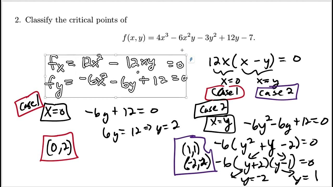
- 🔍 Critical points are identified where the gradient of the function equals zero, resulting in four points: (0,0), (0, -2), (√3, 1), and (-√3, 1).
- 📝 The script explains the use of the second partial derivative test to classify these critical points.
- 📈 The second partial derivatives are computed, including with respect to x twice, y twice, and the mixed partial derivative.
- 🔢 The special second partial derivative test expression is used to classify the critical points, involving the subtraction of the squared mixed partial derivative from the product of the second partial derivatives with respect to x and y.
- 📌 At the point (0,0), the test result is positive, indicating a local maximum due to the negative concavity.
- 📉 For the points (0, -2), (√3, 1), and (-√3, 1), the test results are negative, indicating saddle points.
- 📊 The script emphasizes that the sign of the second partial derivative test expression is crucial for determining the nature of the critical points.
- 📚 The process is explained without the need to visualize the graph, relying solely on mathematical calculations.
- 📝 The script concludes by summarizing that among the four critical points, (0,0) is a local maximum, and the others are saddle points.
- 👋 The video ends with a sign-off, promising to continue the topic in the next video.
Q & A
What are critical points in the context of multivariable calculus?
-Critical points are the points in the domain of a multivariable function where the gradient of the function is equal to zero or is undefined. They are potential candidates for local maxima, minima, or saddle points.
How many critical points were found in the video?
-Four critical points were identified in the video: (0,0), (0, -2), (√3, 1), and (-√3, 1).
What is the second partial derivative test used for?
-The second partial derivative test is used to classify the critical points of a multivariable function. It helps determine whether a critical point is a local maximum, local minimum, or a saddle point.
What are the second partial derivatives computed in the video?
-The second partial derivatives computed in the video are with respect to x twice, with respect to y twice, and the mixed partial derivative term (partial derivative with respect to x and then y or vice versa).
What does the expression for the second partial derivative test consist of?
-The expression for the second partial derivative test consists of the second partial derivative with respect to x squared, multiplied by the second partial derivative with respect to y squared, minus the square of the mixed partial derivative term.
What is the result of the second partial derivative test at the point (0,0)?
-At the point (0,0), the result of the test is positive, indicating a local maximum due to the negative concavity indicated by the second derivative with respect to x.
What does a negative result from the second partial derivative test indicate?
-A negative result from the second partial derivative test indicates a saddle point, as it suggests the function has a different concavity in different directions at that point.
What is the significance of the mixed partial derivative term in the second partial derivative test?
-The mixed partial derivative term is crucial in the second partial derivative test because it helps determine the concavity of the function in two dimensions, which is essential for classifying the critical points.
How many of the critical points found are saddle points according to the video?
-Three of the critical points are saddle points according to the video: (0, -2), (√3, 1), and (-√3, 1).
What is the conclusion about the critical points from the video script?
-The conclusion is that among the four critical points found, (0,0) is a local maximum, and the other three points are saddle points.
Outlines
📚 Introduction to Critical Points and Second Partial Derivative Test
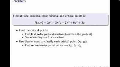
The script begins by reviewing the previous video's task of finding and classifying critical points of a multivariable function. Critical points are identified where the gradient equals zero, resulting in four points: (0,0), (0, -2), (√3, 1), and (-√3, 1). The script then introduces the second partial derivative test for classifying these points. The process involves calculating the second partial derivatives with respect to x and y, and the mixed partial derivative. The script proceeds to demonstrate the calculation of these derivatives for the given function.
🔍 Applying the Second Partial Derivative Test to Critical Points
This paragraph continues the application of the second partial derivative test to classify the critical points. The script explains the formula for the test, which involves the second partial derivatives of the function with respect to x and y, and the subtraction of the square of the mixed partial derivative. The calculations are performed for each critical point, resulting in different values that indicate the nature of the points: a local maximum at (0,0) and saddle points at the other three locations. The script emphasizes the importance of the sign of the result from the test in determining whether a point is a maximum, minimum, or saddle point, and concludes by summarizing the findings without the need for a graph.
Mindmap
Keywords
💡Critical Points
💡Gradient
💡Second Partial Derivative Test
💡Partial Derivatives
💡Concavity
💡Saddle Point
💡Local Maximum/Minimum
💡Mixed Partial Derivative
💡Polynomial Function
💡Second Derivative
Highlights
Introduction to finding and classifying critical points of a multivariable function.
Critical points are identified where the gradient equals zero.
Four critical points were found: (0,0), (0,-2), (√3,1), and (-√3,1).
The second partial derivative test is required to classify critical points.
Partial derivatives of the function are copied and prepared for further use.
Explanation of the process to compute second partial derivatives.
Calculation of the second partial derivative with respect to x.
Derivation of the second partial derivative with respect to y.
Importance of the mixed partial derivative term in the classification process.
Substitution of critical points into the second partial derivative test expression.
Analysis of the result at the point (0,0) indicating a positive value.
Calculation of the second partial derivative test for the point (0,-2) resulting in a negative value.
Substitution of the point (√3,1) into the test yielding a zero value.
Application of the test to the point (-√3,1) resulting in a negative value.
Interpretation of the second partial derivative test results.
Identification of (0,0) as a local maximum based on the test.
Classification of the remaining points as saddle points due to negative test results.
Conclusion that all critical points except (0,0) are saddle points.
The ability to determine the nature of critical points without graphing the function.
Transcripts
Browse More Related Video


5.0 / 5 (0 votes)
Thanks for rating: