Second partial derivative test
TLDRThis video script explores the concept of local minima, maxima, and saddle points in multivariable calculus. It begins with a function f(x, y) and identifies critical points where the gradient equals zero. Using second partial derivatives, the script explains how to determine the nature of these points, highlighting the importance of the mixed partial derivative term. The video introduces the second partial derivative test, illustrating its application with a function that visually demonstrates a saddle point. The script emphasizes the test's utility in discerning between local minima, maxima, and saddle points by analyzing the concavity in different directions.
Takeaways
- 🔍 In the previous video, the function f(x, y) = x^4 - 4x^2 + y^2 was analyzed to find points where the gradient is zero.
- 📍 Three critical points were identified: (0,0), (√2,0), and (-√2,0), with (0,0) being a saddle point and the others local minima.
- 📝 The second partial derivative test was used to explain why (0,0) is a saddle point and the other points are local minima.
- 🔄 Mixed partial derivatives must be considered for a complete analysis of critical points.
- 📊 A new example function, f(x, y) = x^2 + y^2 - 4xy, is introduced, which also has a saddle point at the origin.
- 🔧 Second partial derivatives with respect to x and y were both constant positive two, suggesting a local minimum, but the graph showed a saddle point.
- ❗ The coefficient in front of the xy term affects whether a point is a saddle point or a local minimum.
- 🔀 Changing the coefficient P from 0 to 4 shows a transition from a local minimum to a saddle point.
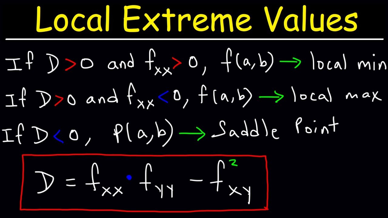
- 📐 The second partial derivative test involves computing H, the product of second partial derivatives with respect to x and y, minus the square of the mixed partial derivative.
- 📉 If H > 0, the point is a local max or min; if H < 0, it is a saddle point; if H = 0, the test is inconclusive.
Q & A
What is the function f(x, y) discussed in the video?
-The function f(x, y) discussed in the video is x^4 - 4x^2 + y^2.
What does it mean for the gradient of a function to be equal to zero?
-For the gradient of a function to be equal to zero means that both partial derivatives with respect to x and y are equal to zero.
What are the three points found where the gradient of the function is zero?
-The three points found are (0, 0), (√2, 0), and (-√2, 0).
What is a saddle point and how does it differ from a local minimum or maximum?
-A saddle point is a point on a surface where the function does not have a local maximum or minimum. It is a point where the concavity in one direction disagrees with the concavity in another direction, unlike a local minimum or maximum where the concavity is consistent in all directions.
What is the significance of the second partial derivatives in determining the concavity of a function?
-The second partial derivatives are used to determine the concavity of a function. A positive second partial derivative indicates concavity upwards (like a smiley face), suggesting a local minimum, while a negative second partial derivative indicates concavity downwards (like a frowny face), suggesting a local maximum.
Why is the mixed partial derivative term important in the second partial derivative test?
-The mixed partial derivative term is important because it can provide additional information about the function's behavior that is not captured by the pure second partial derivatives alone. It can help distinguish between a local minimum, a local maximum, and a saddle point.
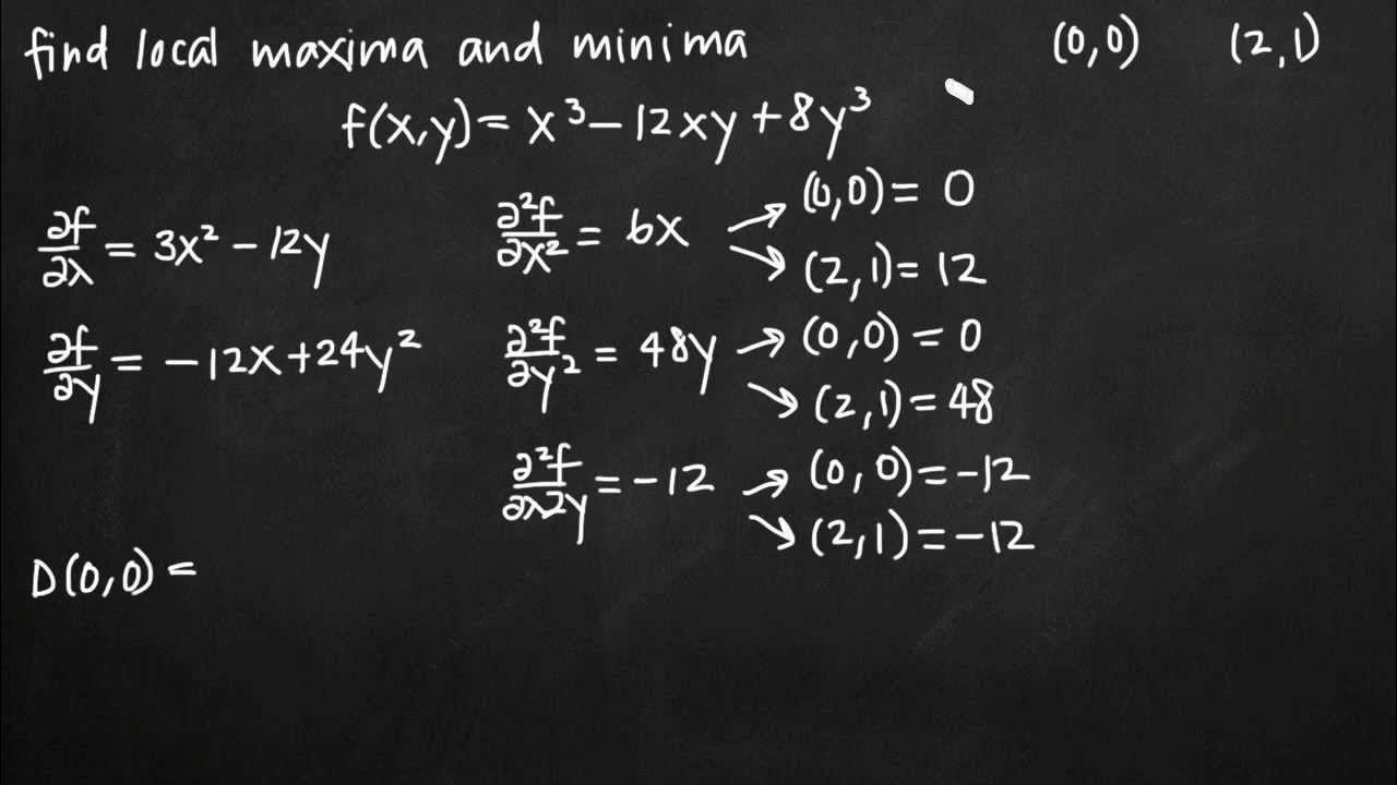
What is the second partial derivative test and how is it used?
-The second partial derivative test is a method used to determine whether a critical point of a function is a local minimum, a local maximum, or a saddle point. It involves calculating a value H using the formula H = f_xx * f_yy - (f_xy)^2, where f_xx is the second partial derivative with respect to x, f_yy is the second partial derivative with respect to y, and f_xy is the mixed partial derivative. The sign of H helps in classifying the critical point.
What does it mean if H is greater than zero in the second partial derivative test?
-If H is greater than zero in the second partial derivative test, it indicates that the function has either a local maximum or a local minimum at the point, but not a saddle point.
What does it mean if H is less than zero in the second partial derivative test?
-If H is less than zero, it indicates that the function has a saddle point at the point, as it suggests that the concavities in different directions disagree.
What is the critical point where H equals zero in the second partial derivative test?
-When H equals zero, the second partial derivative test is inconclusive, meaning it cannot determine whether the point is a local minimum, a local maximum, or a saddle point. This is a special case that requires further analysis.
How does the coefficient in front of the xy term in the function affect the concavity and the nature of the critical points?
-The coefficient in front of the xy term can change the nature of the critical points from local minima to saddle points or vice versa. It influences the sign of H in the second partial derivative test, which in turn affects the classification of the critical points.
Outlines
📚 Gradient and Second Derivative Analysis
This paragraph discusses the analysis of a function's critical points where the gradient is zero, indicating potential local minima, maxima, or saddle points. It explains the process of finding these points by setting partial derivatives to zero and solving for x and y. The function f(x, y) = x^4 - 4x^2 + y^2 is used as an example, and the second partial derivatives are calculated to determine concavity. The mixed partial derivative term is highlighted as crucial for a complete analysis, and a contrasting example with a different function is introduced to illustrate the point.
🔍 The Importance of Mixed Partial Derivatives
This section delves into the significance of mixed partial derivatives in determining the nature of critical points. It uses a function with a graph showing a saddle point at the origin to demonstrate that second partial derivatives alone are insufficient. The function f(x, y) = x^2 + y^2 - 4xy is analyzed, and it's shown that despite positive second partial derivatives, the presence of the -4xy term leads to a saddle point. The paragraph emphasizes the need to consider the mixed partial derivative term in the analysis of critical points.
📘 Introduction to the Second Partial Derivative Test
The paragraph introduces the second partial derivative test, a method for classifying critical points as local minima, maxima, or saddle points. The test involves calculating a value H from the second partial derivatives with respect to x and y, and the mixed partial derivative. If H > 0, the point could be a local maximum or minimum, and further analysis is needed to determine which. If H < 0, the point is a saddle point. If H = 0, the test is inconclusive. The paragraph provides an example using a variable coefficient P in the function to illustrate how the nature of the critical point changes with the value of P, and it explains the critical point where P equals two as a transition from local minimum to saddle point.
🔢 Application of the Second Partial Derivative Test
This final paragraph applies the second partial derivative test to the function from the previous examples, with a focus on the origin as the critical point. It calculates the value H using the previously found second partial derivatives and the mixed partial derivative. The paragraph shows how varying the coefficient P affects the value of H, leading to different classifications of the critical point. It explains the transition from a local minimum to a saddle point as P increases, and the special case when H = 0, which cannot be determined by the test alone.
Mindmap
Keywords
💡Function
💡Gradient
💡Partial Derivatives
💡Saddle Point
💡Local Minima
💡Second Partial Derivatives
💡Mixed Partial Derivative
💡Second Partial Derivative Test
💡Concavity
💡Critical Point
Highlights
The video discusses the function f(x, y) = x^4 - 4x^2 + y^2, identifying critical points where the gradient equals zero.
Three points are found to have zero gradient: (0,0), (2,0), and (-2,0), with the origin being a saddle point and the others local minima.
Second partial derivatives are used to analyze concavity, with a negative result at x=0 indicating a maximum in the x-direction.
The second partial derivative with respect to y is constant and positive, suggesting a minimum in the y-direction.
The importance of considering the mixed partial derivative term for a complete analysis is emphasized.
An example function f(x, y) = x^2 + y^2 - 4xy is introduced to illustrate the limitations of second partial derivatives alone.
The function's partial derivatives at the origin are zero, suggesting a flat tangent plane but not the nature of the point.
Second partial derivatives for the example function suggest positive concavity in both x and y directions, misleadingly indicating a local minimum.
The discrepancy between the graph's saddle point and the second partial derivatives' indication is highlighted.
The coefficient of the xy term is identified as critical in determining whether the point is a local minimum or a saddle point.
A variable P is introduced to demonstrate how the graph changes with different coefficients in front of the xy term.
The second partial derivative test is introduced as a method to determine the nature of a critical point.
The test involves calculating a value H using the second partial derivatives and the mixed partial derivative.
If H > 0, the point could be a maximum or minimum, discerned by analyzing concavity; if H < 0, it is a saddle point.
A special case where H = 0 is mentioned, where the test is inconclusive, though it is rare.
The second partial derivative test is applied to the example function with variable P, illustrating the transition from local minimum to saddle point.
The critical point where the function changes from a local minimum to a saddle point is identified at P = 2.
The video promises to provide more intuition behind the second partial derivative test in a future video.
Transcripts
Browse More Related Video

Second partial derivative test intuition
Second Derivative Test Multivariable (Calculus 3)
Local Extrema, Critical Points, & Saddle Points of Multivariable Functions - Calculus 3
Local extrema and saddle points of a multivariable function (KristaKingMath)
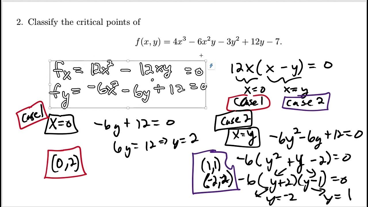
Find and classify critical points

Second partial derivative test example, part 2
5.0 / 5 (0 votes)
Thanks for rating: