Find and classify critical points
TLDRThis video script offers a detailed tutorial on classifying critical points of a function in multivariable calculus. It begins by explaining that critical points occur where partial derivatives with respect to x and y are zero or undefined. The script then demonstrates how to find critical points for a given function by setting the partial derivatives equal to zero and solving for x and y. It introduces two cases based on the solutions and proceeds to classify the critical points using second partial derivatives and the Hessian determinant. The tutorial concludes with identifying one local maximum and two saddle points, providing a clear explanation of how to determine the nature of each critical point using the second derivative test.
Takeaways
- 📚 The concept of critical points in calculus is introduced, distinguishing between Calc 1 and Calc 3 where in Calc 3, partial derivatives are considered.
- 🔍 The partial derivative with respect to x is given as \(12x^2 - 12xy\), and with respect to y as \(-6x^2 - 6y + 12\), which must be set to zero simultaneously to find critical points.
- 📝 Factoring out common terms from the partial derivatives leads to two cases: \(x = 0\) and \(x = y\).
- 📌 For \(x = 0\), solving the resulting equation yields a critical point at \((0, 2)\).
- 🔑 In the case of \(x = y\), solving the quadratic equation derived from the partial derivative with respect to y yields critical points at \((-2, -2)\) and \((1, 1)\).
- 🔍 To classify the critical points, second partial derivatives are needed: \(\frac{\partial^2}{\partial x^2}\), \(\frac{\partial^2}{\partial y^2}\), and the mixed partial \(\frac{\partial^2}{\partial x \partial y}\).
- 📘 The formula for classifying critical points involves the second partial derivatives and is based on the determinant of the Hessian matrix.
- 📊 The determinant \(D\) is calculated for each critical point to determine if it is a local minimum, local maximum, or a saddle point.
- 📈 At the point \((0, 2)\), \(D\) is positive, indicating a local maximum.
- 🐎 The points \((1, 1)\) and \((-2, -2)\) have negative \(D\) values, classifying them as saddle points.
- 📋 The process concludes with a summary of one local maximum at \((0, 2)\) and two saddle points at \((1, 1)\) and \((-2, -2)\).
Q & A
What are the critical points in calculus?
-Critical points in calculus are where the first derivative is equal to zero or undefined. In multivariable calculus, critical points occur where all first partial derivatives with respect to each variable are simultaneously equal to zero.
What is the first partial derivative of the function with respect to x?
-The first partial derivative of the function with respect to x is 12x^2 - 12xy.
What is the first partial derivative of the function with respect to y?
-The first partial derivative of the function with respect to y is -6x^2 - 6y + 12.
How do you find the critical points for the given function?
-To find the critical points, set both first partial derivatives equal to zero simultaneously and solve for the variables x and y.
What are the two cases derived from setting the partial derivative with respect to x equal to zero?
-The two cases derived are when x equals zero and when x equals y.
What is the critical point found when x equals zero?
-When x equals zero, the critical point found is (0, 2).
What are the possible values of y when x equals y?
-When x equals y, the possible values of y are -2 and 1, leading to the critical points (-2, -2) and (1, 1).
What are the second partial derivatives needed to classify the critical points?
-To classify the critical points, you need the second partial derivative with respect to x (f_xx), the second partial derivative with respect to y (f_yy), and the mixed partial derivative (f_xy).
What is the formula used to classify critical points in multivariable calculus?
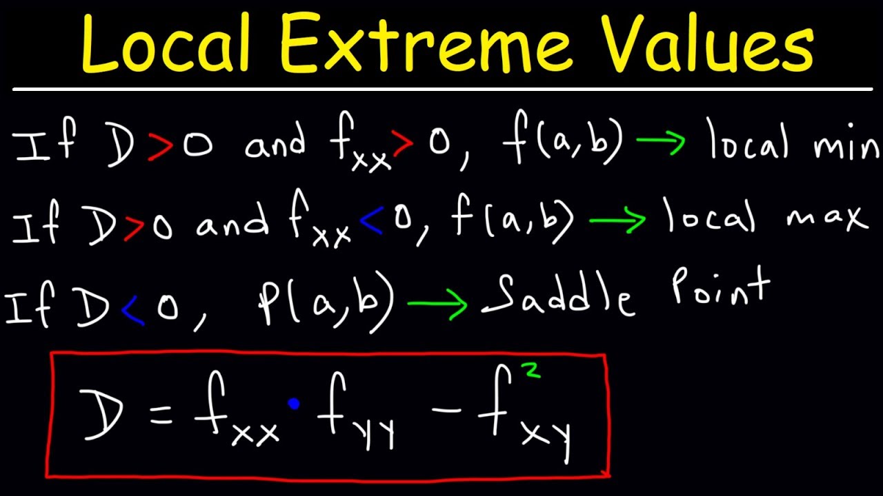
-The formula used to classify critical points is D = (f_xx * f_yy) - (f_xy)^2, which is derived from the determinant of the Hessian matrix.
What does a positive value of D indicate about the critical point?
-A positive value of D indicates that the critical point could be a local minimum or maximum, depending on the sign of the second partial derivative with respect to x (f_xx).
What does a negative value of D indicate about the critical point?
-A negative value of D indicates that the critical point is a saddle point.
How do you determine if a critical point with a positive D value is a local minimum or maximum?
-If the second partial derivative with respect to x (f_xx) is greater than zero, the critical point is a local minimum. If it is less than zero, the critical point is a local maximum.
What are the classifications of the three critical points found in the script?
-The critical point (0, 2) is a local maximum, and the points (-2, -2) and (1, 1) are saddle points.
Outlines
📚 Introduction to Calculus 3 Critical Points
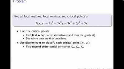
This paragraph introduces the concept of critical points in multivariable calculus, specifically focusing on a function with two variables, x and y. The critical points are identified where the first partial derivatives with respect to x and y are either equal to zero or undefined. The function provided has partial derivatives of 12x^2 - 12xy for x and -6x^2 - 6y + 12 for y. The task is to set these partial derivatives equal to zero simultaneously and solve for x and y, leading to two cases: x equals zero and x equals y.
🔍 Solving for Critical Points and Their Classification
The paragraph delves into solving for the critical points of the given function. For the case where x equals zero, it is determined that y must be 2, resulting in the critical point (0, 2). For the case where x equals y, a quadratic equation is formed and solved, yielding two more critical points: (-2, -2) and (1, 1). The paragraph then explains the process of classifying these critical points using second partial derivatives. A formula involving the second partial derivatives (D) is introduced, which is derived from the Hessian matrix. By evaluating D at each critical point, one can determine if the point is a local minimum, local maximum, or a saddle point.
📉 Determining the Nature of Critical Points Using the Hessian
This final paragraph concludes the process by evaluating the Hessian determinant (D) at the found critical points to classify them. At the point (0, 2), D is positive, indicating a local maximum. At the points (-2, -2) and (1, 1), D is negative, signifying saddle points. The paragraph further explains the concept of saddle points as points that appear as a maximum when viewed from one direction and a minimum from another, akin to the shape of a saddle. It also clarifies that a positive D value at (0, 2) could indicate either a local minimum or maximum, but the second derivative test (double x) reveals it to be a local maximum since it is negative. The summary ends with a recap of the method to find and classify critical points in multivariable calculus.
Mindmap
Keywords
💡Critical Points
💡First Derivative
💡Partial Derivatives
💡Factoring
💡Quadratic Equation
💡Second Partials
💡Hessian Matrix
💡Determinant
💡Saddle Point
💡Local Min/Max
Highlights
Critical points in calculus are identified where the first derivative is zero or undefined.
In multivariable calculus, critical points are found where partial derivatives with respect to each variable are zero simultaneously.
The partial derivative with respect to x is 12x^2 - 12xy.
The partial derivative with respect to y is -6x^2 - 6y + 12.
Factoring out common terms from the partial derivatives leads to x - y = 0.
Two cases arise: x = 0 and x = y.
If x = 0, solving the equations yields the critical point (0, 2).
If x = y, solving the quadratic equation yields y = -2 or y = 1, leading to critical points (-2, -2) and (1, 1).
Second partial derivatives are needed to classify the critical points: d^2/dx^2, d^2/dy^2, and mixed partial d^2/dxdy.
The second partial derivatives are calculated as 24x - 12y for d^2/dx^2 and -6 for d^2/dy^2.
The mixed partial is the derivative of the partial with respect to y of the partial with respect to x, which equals -12x.
A determinant formula involving second partials, known as the Hessian, is used to classify critical points.
Evaluating the determinant at the critical points helps in classifying them as local minima, maxima, or saddle points.
At the point (0, 2), the determinant is positive, indicating a local maximum.
At the points (-2, -2) and (1, 1), the determinant is negative, indicating saddle points.
The second partial with respect to x alone can also indicate concavity and thus classify a local minimum or maximum.
The process of classifying critical points involves setting first partial derivatives to zero, solving for variables, and then using second partials to determine the nature of the critical points.
Transcripts
Browse More Related Video
Critical Points of Functions of Two Variables

Second partial derivative test example, part 1
Local Extrema, Critical Points, & Saddle Points of Multivariable Functions - Calculus 3

Use the Second Derivative Test to Find Any Extrema and Saddle Points: f(x,y) = -4x^2 + 8y^2 - 3

Oxford Calculus: Finding Critical Points for Functions of Two Variables

Second partial derivative test
5.0 / 5 (0 votes)
Thanks for rating: