Lagrange Multipliers with TWO constraints | Multivariable Optimization
TLDRThis video explores the concept of LaGrange multipliers with two constraints, a powerful tool for optimizing multivariable functions. The presenter explains the algebraic and geometric aspects of the method using an example that involves minimizing the distance from the origin to points on the intersection of two surfaces. The video demonstrates solving a system of equations involving gradients and constraints to find extrema points, and uses GeoGebra to visually interpret the solution, ultimately identifying the closest and furthest points from the origin.
Takeaways
- 📚 The video introduces the concept of LaGrange multipliers, a mathematical method for optimizing multivariable functions subject to constraints.
- 🔍 LaGrange multipliers are powerful for dealing with multiple constraints, which is the focus of the video, expanding on a previous video that covered a single constraint.
- 📈 The video aims to provide both an algebraic and geometric understanding of the LaGrange multipliers through an example.
- 📝 The example involves optimizing a function \( f(x, y, z) \) subject to two constraints \( G_1 = 0 \) and \( G_2 = 0 \), where the function represents the distance squared from the origin.
- 📐 The script explains that the intersection of two constraint surfaces typically forms a curve, which is the set of points where both constraints are satisfied simultaneously.
- 📉 The LaGrange multiplier system involves setting up an equation where the gradient of the function to be optimized is proportional to a linear combination of the gradients of the constraints.
- 🔢 The video provides a step-by-step algebraic solution to the example problem, demonstrating how to derive and solve the system of equations resulting from the LaGrange multiplier method.
- 📍 The script identifies two potential solutions (extrema points) for the example problem by analyzing the system of equations derived from the LaGrange multipliers.
- 📊 The video uses GeoGebra to visually represent the constraints, the intersection curve, and the function to be optimized, providing a geometric interpretation of the problem.
- 🔎 It is shown that one of the points corresponds to the minimum distance from the origin to the intersection curve, while the other corresponds to the maximum distance.
- 🎯 The video concludes by demonstrating the use of spheres in GeoGebra to visually identify the points of minimum and maximum distance from the origin on the intersection curve.
Q & A
What are the LaGrange multipliers?
-LaGrange multipliers are a mathematical method for finding the local maxima and minima of a function subject to equality constraints. They are particularly useful for optimizing multivariable functions with multiple constraints.
Why are LaGrange multipliers powerful in optimization problems?
-LaGrange multipliers are powerful because they allow for the optimization of multivariable functions while considering multiple constraints, which is often necessary in real-world problems.
What is the geometric interpretation of LaGrange multipliers?
-Geometrically, LaGrange multipliers find points where the gradient of the function to be optimized is parallel to the gradients of the constraint functions, which represent the intersection of the constraint surfaces.
How does the video script introduce the concept of LaGrange multipliers with two constraints?
-The script introduces the concept by first explaining the case with a single constraint and then extending it to two constraints, emphasizing the intersection of two surfaces and the use of gradients to form a plane that is normal to the intersection curve.
What is the significance of the gradients of G1 and G2 in the context of LaGrange multipliers?
-The gradients of G1 and G2 are significant because they define a plane that contains all possible directions normal to the intersection curve of the two constraint surfaces, which is where the optimization occurs.
What is the system of equations that defines the LaGrange multipliers for two constraints?
-The system of equations for two constraints includes the vector equation where the gradient of the function F is equal to lambda times the gradient of G1 plus mu times the gradient of G2, along with the equations G1=0 and G2=0.
How does the script use an example to illustrate the application of LaGrange multipliers?
-The script uses an example of optimizing the distance from the origin to points on the intersection of two constraints, providing both algebraic and geometric interpretations of the process.
What is the function being optimized in the provided example?
-In the example, the function being optimized is the distance squared from the origin to any point on the intersection of the two constraints, represented by x^2 + y^2 + z^2.
How does the script simplify the problem of finding extrema using LaGrange multipliers?
-The script simplifies the problem by breaking down the vector equation into three standard equations based on the partial derivatives with respect to x, y, and z, and then solving these equations along with the constraint equations.
What tool does the script mention for visualizing the optimization problem?
-The script mentions GeoGebra as a tool for visualizing the optimization problem, allowing students to graph different plots and see the intersection of constraint surfaces.
How does the script use spheres to visualize the minimization of distance in the example?
-The script uses spheres of varying radii to represent the distance squared from the origin and shows how these spheres intersect with the ellipse formed by the intersection of the two constraints, helping to visualize the closest and furthest points.
Outlines
📚 Introduction to LaGrange Multipliers with Multiple Constraints
This paragraph introduces the concept of LaGrange multipliers, a mathematical tool used for optimizing multivariable functions under multiple constraints. The speaker explains that LaGrange multipliers are powerful for dealing with optimization problems where the function to be optimized is subject to multiple constraints that must be simultaneously satisfied. The explanation includes a visual representation of constraints as surfaces intersecting along a curve, which is the set of points where the optimization will be performed. The paragraph sets the stage for a deeper dive into the algebraic and geometric aspects of the LaGrange multipliers method.
🔍 Setting up the LaGrange Multipliers System for Optimization
The speaker delves into the algebraic formulation of the LaGrange multipliers system, starting with a review of the single-constraint case and then moving on to the more complex scenario of two constraints. The paragraph explains the process of setting up the system of equations that includes the gradients of the objective function and the constraints, weighted by the LaGrange multipliers. The speaker illustrates this with an example of optimizing the distance from the origin to points on the intersection of two surfaces defined by constraints G1 and G2. The gradients of these constraints and the objective function are used to form a system of equations that will be solved to find the optimal points.
📉 Solving the System of Equations for Optimal Points
This section focuses on solving the system of equations derived from the LaGrange multipliers method. The speaker simplifies the system by identifying equations that can be easily satisfied and then explores different cases based on these simplifications. The process involves substituting values and solving for variables x, y, and z, which represent the coordinates of the points on the intersection curve. The speaker also discusses the geometric interpretation of these points as potential maxima or minima of the distance function subject to the given constraints.
📊 Geometrical Interpretation and Visualization Using GeoGebra
The final paragraph wraps up the discussion by providing a geometrical interpretation of the results obtained from the LaGrange multipliers method. The speaker uses GeoGebra, a mathematical visualization tool, to graph the constraints and the intersection curve, as well as the spheres representing different distances from the origin. This visual approach helps to identify the points of minimum and maximum distance from the origin on the intersection curve. The speaker demonstrates how to adjust the radius of the spheres to find the points of intersection with the ellipse, which correspond to the optimal solutions for the given optimization problem.
Mindmap
Keywords
💡Lagrange Multipliers
💡Multivariable Functions
💡Constraints
💡Gradient
💡Level Surfaces
💡Optimization
💡Normal Vector
💡Intersection Curve
💡Algebraic Solution
💡Geometrical Interpretation
💡Distance Function
Highlights
Introduction to the concept of Lagrange multipliers in the context of multivariable functions with multiple constraints.
Explanation of the power of Lagrange multipliers for optimization problems involving multiple constraints.
Visual representation of the intersection of two surfaces, typically represented as a curve, in the context of constraints.
Identification of normal vectors to the constraint surfaces using the gradients of the constraint functions.
Derivation of the Lagrange multiplier system of equations for two constraints, involving lambda and mu parameters.
Example problem setup involving optimizing the distance from the origin to points on the intersection of two constraints.
Implicit function representation of the distance squared as the objective function for optimization.
Formulation of the gradient equations for the objective function and constraints using partial derivatives.
Solving the system of equations algebraically to find potential extrema points.
Case analysis to simplify the system and find possible values for x, y, z, lambda, and mu.
Identification of two candidate points as potential extrema of the distance function under constraints.
Evaluation of the function values at the candidate points to determine which is a minimum and which is a maximum.
Use of GeoGebra to visually interpret the optimization problem and the intersection of constraints.
Graphical representation of the constraints as cones and a plane, and their intersection as an ellipse.
Visualization of the distance function as a sphere and its intersection with the ellipse to find extrema.
Demonstration of the practical application of Lagrange multipliers using GeoGebra for a geometric understanding.
Conclusion summarizing the process and results of using Lagrange multipliers for the given optimization problem.
Transcripts
Browse More Related Video
Calculus 3: Lagrange Multipliers (Video #18) | Math with Professor V

Lagrange Multipliers | Geometric Meaning & Full Example

BusCalc 14.4 Lagrange Multipliers

Lec 13: Lagrange multipliers | MIT 18.02 Multivariable Calculus, Fall 2007

Lagrange Multipliers
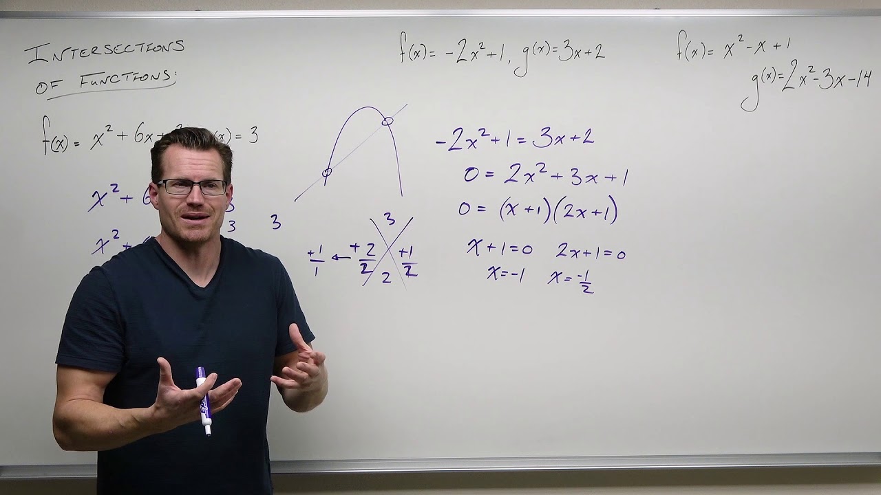
Finding Intersections of Functions (Precaluclus - College Algebra 22)
5.0 / 5 (0 votes)
Thanks for rating: