BusCalc 14.4 Lagrange Multipliers

Drew Macha

4 May 202268:37

EducationalLearning

32 Likes 10 Comments

TLDRThe transcript details a comprehensive lesson on the application of the method of Lagrange multipliers for optimizing multi-variable functions subject to constraints. The lecturer begins by illustrating the process of finding critical points of a function and characterizing them as maximum, minimum, or saddle points using first and second derivatives. They then delve into the method of Lagrange multipliers, explaining the setup of the Lagrange function, involving the objective function, the constraint function, and the introduction of a new variable, lambda. The process involves finding the partial derivatives with respect to each variable and solving a system of equations to find the optimal points that satisfy the constraint. The lecturer provides two detailed examples, demonstrating how to apply the method to find maximum and minimum values of functions under specific constraints. The examples include visualizing the function's behavior using contour lines and understanding how the method can be applied in real-world scenarios, such as optimizing flow rates in a chemical plant. The lesson concludes with a discussion on the practical applications of the method in industry and business, emphasizing its significance in solving optimization problems with constraints.

Takeaways

📚 The process of finding critical points of a function involves taking the first and second derivatives, setting them equal to zero, and solving the system of equations.
🔍 To determine the nature of a critical point (maximum, minimum, or saddle point), calculate the value of 'M' which is the product of f_xx * f_yy - f_xy^2, where f_xx, f_yy, and f_xy are the second derivatives and the mixed partial derivative.
📉 A positive 'M' value indicates a minimum at the critical point, a negative 'M' suggests a saddle point, and 'M' equal to zero means the test is inconclusive.
🔑 The method of Lagrange multipliers is used to optimize multi-variable functions while adhering to constraints, which is particularly useful in real-world applications.
📐 The Lagrange function, F(X, Y, λ), is constructed by combining the function to be optimized with the constraint equation multiplied by a new variable, the Lagrange multiplier (λ).
🧮 Partial derivatives of the Lagrange function with respect to each variable (including λ) are set to zero, forming a system of equations to solve for the variables.
🔍 The constraint equation must be arranged so that one side equals zero for the method of Lagrange multipliers to work.
🔢 Solving the system of equations from the Lagrange function can yield multiple points, which may represent different types of extrema (maximums or minimums) along the constraint.
📈 Contour lines on a graph can help visualize the behavior of a function and its critical points relative to the constraint.
🔬 Lagrange multipliers have practical applications in various industries, such as chemical plants, where they can be used to optimize processes subject to physical constraints like mass conservation.
⏱️ The method can be computationally intensive but is valuable for solving complex optimization problems with constraints, as demonstrated in the example of an oil refinery with thousands of flow meters.

Q & A

What is the main topic discussed in the transcript?
-The main topic discussed in the transcript is the method of Lagrange multipliers, which is used to optimize multi-variable functions while adhering to certain constraints.
What are the steps involved in using the method of Lagrange multipliers?
-The steps involved are: 1) Writing the Lagrange function with the function to be optimized and the constraint, 2) Calculating the partial derivatives of the Lagrange function with respect to each variable, 3) Solving the system of equations formed by setting these partial derivatives to zero along with the constraint equation, and 4) Analyzing the solutions to determine if they correspond to maxima, minima, or saddle points.
How does the method of Lagrange multipliers help in real-world applications?
-The method of Lagrange multipliers is useful in real-world applications where optimization is required under constraints, such as in chemical plants for optimizing flow rates while conserving mass, or in business for maximizing profit subject to certain limitations.
What is a critical point in the context of the given transcript?
-A critical point is a point in the domain of a function where all the first-order partial derivatives are simultaneously zero. These points are potential candidates for local maxima, minima, or saddle points of the function.
How can you determine if a critical point corresponds to a maximum, minimum, or saddle point?
-You can determine the nature of a critical point by calculating the second-order partial derivatives and the mixed partial derivative at that point. Using these, you compute the value of the determinant of the Hessian matrix, denoted as 'M' in the transcript. If 'M' is positive and the second derivative with respect to x is positive, it's a minimum. If 'M' is negative, it's a saddle point. If 'M' is zero, the test is inconclusive.
What is the significance of the 'M' value in characterizing a critical point?
-The 'M' value is a determinant that is used to determine whether a critical point is a maximum, minimum, or saddle point. It is computed from the second-order partial derivatives and the mixed partial derivative at the critical point.
What is a contour line in the context of the function being optimized?
-A contour line represents a level curve on the graph of a function, where all points on the curve have the same function value. In the context of the transcript, contour lines are used to visualize the function's levels of z-values and how they intersect with the constraint.
How does the constraint affect the optimization process?
-The constraint limits the domain of the function to a specific region. Optimization under constraints means finding the maximum or minimum values of the function only within the region defined by the constraint, rather than over the entire domain of the function.
What is the role of lambda in the method of Lagrange multipliers?
-Lambda, often denoted by the Greek letter λ, is a multiplier used in the Lagrange function to adjust the function in such a way that it satisfies the constraint while optimizing (maximizing or minimizing) the function.
Why is it necessary to set one side of the constraint equation to zero?
-Setting one side of the constraint equation to zero simplifies the formulation of the Lagrange function. It ensures that the constraint can be directly incorporated into the system of equations that need to be solved to find the optimal solution.
What is the purpose of visualizing the function and its constraint using contour lines and a 3D graph?
-Visualizing the function and its constraint helps to understand the shape of the function's surface and how the constraint affects the region over which optimization is performed. It assists in identifying where the maximum or minimum values are likely to occur in relation to the constraint.

Outlines

00:00

📚 Calculus: Finding Critical Points and Derivatives

The first paragraph introduces the process of finding critical points of a function by taking its first and second derivatives. The speaker uses subscript notation and calculates the first and second derivatives with respect to x and y, including the mixed partial derivative. The critical points are found by setting these derivatives equal to zero, forming a system of two equations with two unknowns, which are then solved to find a single critical point at (-7, 8).

05:01

🔍 Characterizing Critical Points and the Method of Lagrange Multipliers

The second paragraph discusses characterizing the found critical point as a maximum, minimum, or saddle point. This involves calculating the second derivatives (fxx, fyy) and the mixed partial derivative at the critical point to form an expression 'M'. The sign of 'M' and the second derivatives help determine the nature of the critical point. The paragraph also introduces the concept of the method of Lagrange multipliers for optimizing multi-variable functions with constraints.

10:01

📐 Setting Up the Lagrange Function and Solving for Unknowns

The third paragraph explains how to set up the Lagrange function with an example of optimizing the function x^2 - y^2 subject to the constraint (x - 1)^2 + (y - 1)^2 = 4. The process involves writing the Lagrange function, calculating partial derivatives, and solving a system of three equations with three unknowns (x, y, and λ, the Lagrange multiplier). The solution process is demonstrated step by step.

15:06

🔢 Solving the System of Equations for the Lagrange Multiplier

The fourth paragraph continues the example from the previous paragraph, focusing on solving the system of equations for the Lagrange multiplier λ. The process involves algebraic manipulation and substitution to simplify the equations and isolate λ, which is then solved to find the values that satisfy the constraint and optimize the function.

20:10

🔍 Analyzing the Function's Maximum and Minimum Values

The fifth paragraph describes the analysis of the function's maximum and minimum values along the constraint. The speaker uses contour lines to visualize the function's behavior and to estimate the location of the maximum and minimum values. The method of Lagrange multipliers is applied to find the exact points where the maximum and minimum values occur subject to the constraint.

25:16

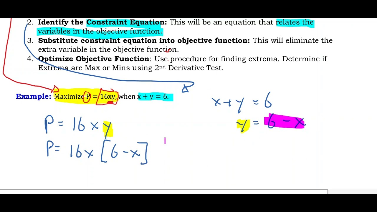
📐 Applying the Method of Lagrange Multipliers to a Paraboloid

The sixth paragraph applies the method of Lagrange multipliers to find the minimum or maximum of a paraboloid function subject to a linear constraint. The constraint represents a line, and the function is a bowl-shaped paraboloid. The process simplifies to finding a point (1,1) that satisfies both the function's optimization and the constraint equation, which is visualized through the contour lines of the paraboloid.

30:17

🌐 Real-World Application of Lagrange Multipliers

The seventh paragraph discusses a real-world application of the method of Lagrange multipliers in the context of a chemical plant. The speaker describes a scenario where mass flow rates are measured and need to be optimized subject to physical constraints, such as mass conservation. The method is used to adjust measured values to fit the physical constraints, resulting in a meaningful optimization within the system.

35:24

📝 Wrapping Up and Preparing for the Exam

The final paragraph wraps up the discussion and prepares students for an upcoming exam. The speaker offers to review problem-solving techniques and concepts, encourages students to come with questions, and emphasizes the applicability and difficulty of the method of Lagrange multipliers in various fields.

Mindmap

Keywords

💡Derivatives

Derivatives are mathematical expressions that represent the rate at which a function changes with respect to a variable. In the video, derivatives are used to find critical points of a function, which are essential for determining the function's maximum or minimum values. The first derivative indicates the slope of the tangent to the function, while the second derivative provides information about the concavity of the function.

💡Critical Points

Critical points are the points on a function where the first derivative is zero or undefined. They are significant because they often correspond to local maxima, minima, or saddle points. In the video, the process of finding critical points involves setting the first derivatives equal to zero and solving for the variables, which helps in identifying potential extrema of the function.

💡Second Derivative Test

The second derivative test is a method used to determine whether a critical point is a maximum, minimum, or neither. It involves evaluating the second derivative of the function at the critical point. If the second derivative is positive, the point is a local minimum; if it's negative, it's a local maximum; and if it's zero, the test is inconclusive. In the video, the second derivative test is applied to classify the critical point found at (-7, 8) as a minimum.

💡Lagrange Multipliers

Lagrange multipliers is a method used in optimization problems where you want to maximize or minimize a function subject to constraints. It involves forming a Lagrange function that includes the original function, the constraints, and a new variable called the Lagrange multiplier. In the video, this method is used to find the maximum and minimum values of a function subject to a constraint, such as finding the maximum value of x^2 - y^2 on a circle in the xy-plane.

💡Contour Lines

Contour lines are lines on a graph that represent points of equal value of a function. They are used to visualize the function's level curves and help in understanding the function's shape and behavior. In the video, contour lines are used to visualize the function x^2 - y^2 and its behavior subject to the constraint of a circle, aiding in the identification of maximum and minimum points.

💡Method of Optimization

The method of optimization refers to the process of finding the maximum or minimum values of a function. It is a fundamental concept in calculus with applications in various fields. In the video, the method of optimization is discussed in the context of finding extrema of functions with constraints, using both the second derivative test and the method of Lagrange multipliers.

💡Constraint

A constraint is a condition or restriction that limits the solution set of an optimization problem. In the context of the video, constraints are represented by equations that the variables of the function must satisfy. For example, the constraint x + y - 2 = 0 limits the values of x and y to lie on a line, and the optimization problem seeks to find the maximum or minimum of the function within this line.

💡Partial Derivatives

Partial derivatives are derivatives of a function with respect to one variable while keeping other variables constant. They measure the rate of change of a function in a particular direction. In the video, partial derivatives are calculated for both x and y to find the critical points and are used in setting up the system of equations in the method of Lagrange multipliers.

💡Multivariable Function

A multivariable function is a function that has more than one independent variable. For example, f(x, y) = x^2 - y^2 is a multivariable function of x and y. In the video, multivariable functions are optimized subject to constraints, and the process involves finding critical points and using the method of Lagrange multipliers.

💡Saddle Point

A saddle point is a point on a surface where the function has a local minimum in one direction and a local maximum in another direction. It is not a local extremum in a single variable context. In the video, the concept of a saddle point is mentioned in relation to the function x^2 - y^2, which has a saddle point at the origin (0,0).

💡System of Equations

A system of equations is a set of two or more equations that need to be solved simultaneously. In the context of the video, a system of equations is formed by setting the partial derivatives equal to zero and including the constraint equation. Solving this system yields the values of the variables that correspond to the critical points of the function.

Highlights

The concept of finding first and second derivatives of a function to identify critical points.

Using subscript notation to simplify the representation of the function, denoted as 'f'.

Process of differentiating the function with respect to x and y, treating the other variable as a constant.

Calculation of second derivatives and mixed partial derivatives to analyze the function's behavior.

Determination of critical points where both first derivatives equal zero, leading to a system of equations.

Solving the system of equations by substitution and simplification to find the critical point.

Characterization of the critical point using the second derivative test to discern if it's a maximum, minimum, or saddle point.

Explanation of the method of Lagrange multipliers for optimizing multi-variable functions with constraints.

Procedure of setting up the Lagrange function with an additional variable, lambda, representing the multiplier.

Taking partial derivatives of the Lagrange function with respect to each variable and setting them to zero.

Solving the system of equations resulting from the method of Lagrange multipliers to find optimal points.

Application of the method to real-world problems, such as optimizing flow rates in a chemical plant.

Use of the method to ensure physical constraints, like mass conservation, are met in optimization problems.

The method's applicability in various industries and business scenarios for optimization under constraints.

Example of finding maximum or minimum values of a function subject to the constraint of a circle on the xy-plane.

Visual approach to understanding the optimization problem by plotting contour lines and the constraint circle.

Detailed walkthrough of solving a complex optimization problem using the method of Lagrange multipliers.

Substitution and simplification techniques to handle complex equations arising from the method.

Utilization of a calculator to find approximate values for the variables in the optimization problem.

Identification of multiple potential maximum or minimum points and the need for context clues to determine their nature.

Transcripts

Browse More Related Video

Lagrange Multipliers

Lec 13: Lagrange multipliers | MIT 18.02 Multivariable Calculus, Fall 2007

Lagrange Multipliers | Geometric Meaning & Full Example

Calculus 3: Lagrange Multipliers (Video #18) | Math with Professor V

Introduction to Optimization

❖ LaGrange Multipliers - Finding Maximum or Minimum Values ❖

Related Tags

Lagrange Multipliers Optimization Multi-variable Functions Derivatives Contour Lines Critical Points Mathematical Analysis Physical Applications Engineering Chemical Plant Flow Meters