Elementary Stats Lesson #20
TLDRThis video script covers the statistical techniques for comparing two population proportions, essential for analyzing differences between groups. It introduces the concept of sampling distribution and the central limit theorem for proportions. The lesson explains how to construct hypothesis tests and confidence intervals for the difference between two proportions, using the pooled estimate of p and standard error calculation. The script also demonstrates the application of these methods through various examples, including testing hypotheses and calculating confidence intervals, ultimately empowering viewers to perform comparative statistical analysis.
Takeaways
- 📚 The lesson introduces chapter 11, focusing on statistical techniques for two-sample inference for population proportions.
- 🔄 A correction is made, clarifying that the lesson is number 20, not 18 or 19 as previously stated.
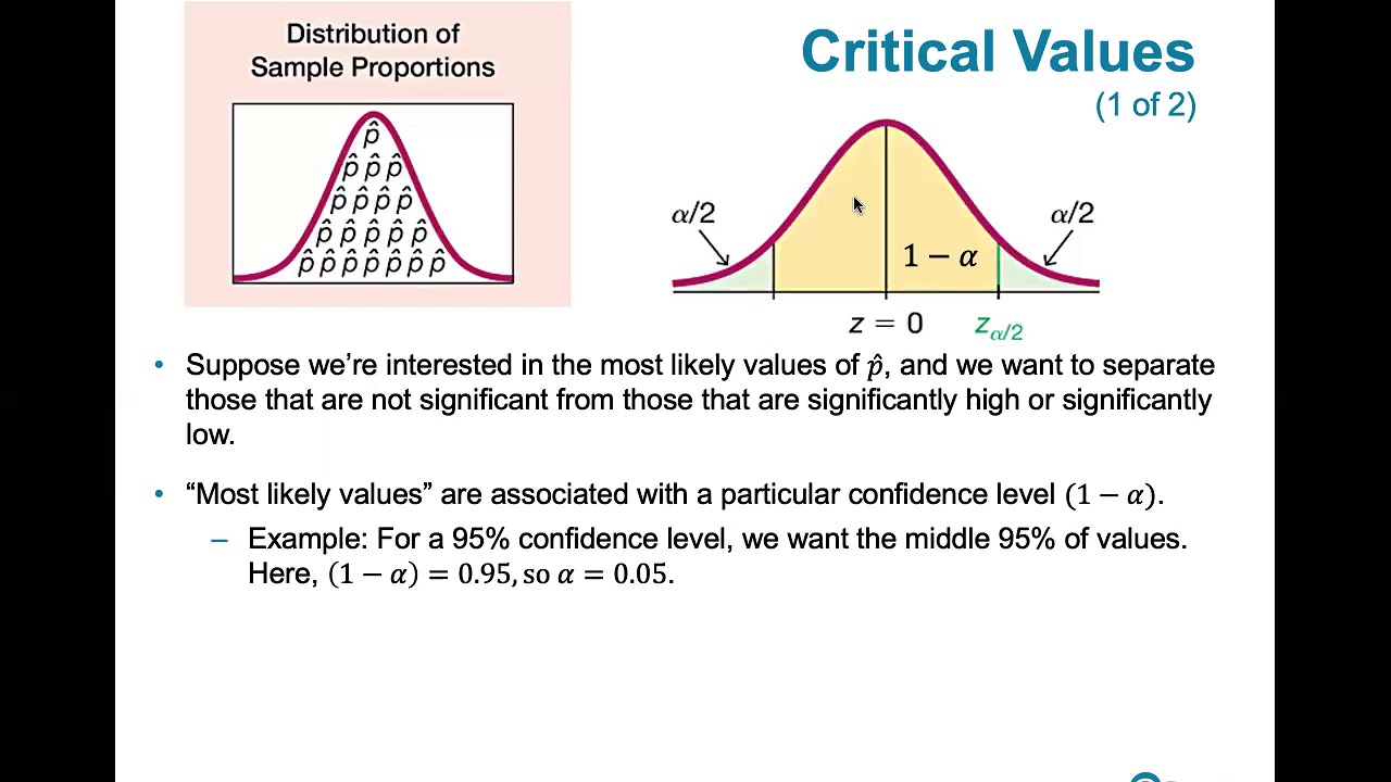
- 📈 The central limit theorem is fundamental, stating that the sampling distribution of the sample proportion (p-hat) is approximately normally distributed with mean equal to the population proportion (p) and a standard error based on the sample size.
- 📝 The point estimate for a population proportion is given by the sample proportion (p-hat), calculated as the number of successes (x) divided by the sample size (n).
- 🧐 Two-sample inference allows for the comparison of proportions between two different treatments or populations, with the new parameter of interest being the difference in proportions (p1 - p2).
- 🤔 The test statistic for comparing two proportions is derived, assuming the null hypothesis that the proportions are equal, and involves a standard score (z-score) based on the difference in sample proportions and their standard error.
- 📉 The null hypothesis for two-sample proportion problems always states that the population proportions are equal, which implies the difference between them is zero.
- 🔢 The pooled estimate of the common proportion (p-hat) is used as a substitute in the test statistic formula when the actual common proportion is unknown, calculated from the combined successes and sample sizes of both groups.
- 📊 The test statistic formula for comparing two population proportions includes the difference in sample proportions, the pooled estimate, and the reciprocals of the sample sizes.
- 📉 The script provides an example of testing the claim that urban households have a higher percentage of internet access than rural households using a hypothesis test at the 5% significance level, concluding no significant difference.
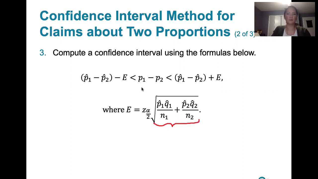
- 📝 The lesson also covers how to construct a confidence interval for the difference between two population proportions, using the same principles of hypothesis testing but focusing on estimating the actual difference.
Q & A
What is the main topic of chapter 11 in the transcript?
-The main topic of chapter 11 is two-sample inference for population proportions, which allows for the comparison of two different treatments or populations in terms of their proportions for some characteristic.
What is the point estimate for a population proportion based on the transcript?
-The point estimate for a population proportion is given by the sample proportion (p hat), where x represents the number of successes and n is the sample size from a simple random sample.
What is the central limit theorem for proportions as mentioned in the transcript?
-The central limit theorem for proportions states that the sampling distribution of the sample proportion (p hat) is approximately normally distributed with the center at the population proportion and the standard error given by the square root of (p * (1 - p)) / n, provided the sample size is large enough.
What is the test statistic used for hypothesis testing with one sample proportion according to the transcript?
-The test statistic used for hypothesis testing with one sample proportion is a z-score (z naught), which is calculated as the sample proportion minus the null proportion divided by the standard error estimate, assuming the null hypothesis is true.
How is the sampling distribution of the difference between two sample proportions described in the transcript?
-The sampling distribution of the difference between two sample proportions (p1 hat minus p2 hat) is approximately normal with the center at the true difference between population proportions (p1 minus p2) and the standard deviation calculated using a square root formula that incorporates both sample sizes and their respective proportions.
What is the null hypothesis for two-sample proportion problems as stated in the transcript?
-The null hypothesis for two-sample proportion problems is that the population proportion of group one is equal to the population proportion of group two (p1 = p2), which implies there is no difference between the two groups.
What is the pooled estimate of p used in the test statistic formula for comparing two population proportions?
-The pooled estimate of p is used as a substitution for the common proportion in the test statistic formula when the null hypothesis is assumed to be true. It is calculated by combining all successes from both samples and dividing by the total number of individuals sampled from both populations.
How is the test statistic formula for comparing two population proportions simplified in the transcript?
-The test statistic formula is simplified by removing the minus zero from the difference in sample proportions (p1 hat - p2 hat) and separating out the square root to include the common proportion and the sum of the reciprocals of the sample sizes.
What is the significance of the common proportion p in the test statistic formula for two sample proportions?
-The common proportion p is significant because it represents the assumed equal value of p1 and p2 under the null hypothesis. It is used in the standard error calculation of the test statistic to account for the uncertainty in the difference between the two sample proportions.
How does the transcript describe the process of constructing a confidence interval for the difference between two population proportions?
-The process involves ensuring random sampling, checking that both sample sizes are sufficiently large (using the condition n * p * (1 - p) > 10), and ensuring both samples stay under 5% of the population for independence. The confidence interval is then constructed using the point estimate (p1 hat - p2 hat), the critical value from the z-distribution, and the standard error estimate.
What is the purpose of the calculator method mentioned in the transcript for hypothesis testing with two sample proportions?
-The calculator method simplifies the process of hypothesis testing by automating the calculations for the test statistic and p-value, reducing the potential for manual calculation errors and providing quick results.
How does the transcript illustrate the application of the two-sample proportion test using an example about internet access?
-The transcript uses an example where an economist wants to test if the percentage of urban households with internet access is greater than that of rural households. It demonstrates setting up the hypothesis, calculating the test statistic, determining the p-value, and making a conclusion based on the comparison of the p-value with the significance level.
What are the conditions for constructing a confidence interval for the difference between two population proportions as outlined in the transcript?
-The conditions include having random samples, both sample sizes must be sufficiently large (n * p * (1 - p) > 10 for both samples), and both samples must be less than 5% of the population to ensure independence.
How does the transcript explain the process of hypothesis testing for two population proportions using a calculator program?
-The transcript describes using a calculator program labeled as 'two prop z test' which automates the process of hypothesis testing. It requires inputting the sample data, specifying the alternate hypothesis, and then calculating to obtain the test statistic and p-value.
What is the conclusion of the hypothesis test about internet access in the transcript?
-The conclusion is that the p-value (0.0918) is greater than the significance level (0.05), so the null hypothesis is not rejected. This means there is insufficient statistical evidence to conclude that there is a difference between the proportions of urban and rural households with internet access.
What is the purpose of the 'two prop z interval' calculator program mentioned in the transcript?
-The 'two prop z interval' calculator program is used to construct a confidence interval for the difference between two population proportions, providing a range within which the true difference is likely to fall with a certain level of confidence.
How does the transcript describe the process of hypothesis testing for two population proportions when the null hypothesis is that p1 is less than p2?
-The transcript describes setting up a left-tailed test, using the 'two prop z test' calculator program, and interpreting the test statistic and p-value to determine whether there is sufficient statistical evidence to support the alternate hypothesis that p1 is less than p2.
What is the conclusion of the hypothesis test for the difference in proportions between two earning groups regarding the moral acceptability of unwed women having children?
-The conclusion is that there is a statistically significant difference between the proportions of the two earning groups, as the confidence interval does not include zero, indicating that the difference in their views on the moral acceptability of unwed women having children is likely real.
What is the next topic to be covered after the two-sample proportion tests as mentioned in the transcript?
-The next topic to be covered is how to compare two different means from two different groups and how to capture the value of the difference between these means, which will involve discussing t-procedures.
Outlines
📚 Introduction to Chapter 11: Two Sample Inference for Proportions
The instructor begins by correcting a previous error regarding the lesson number and introduces chapter 11, which focuses on two sample inference for population proportions. This technique is crucial for comparing two treatments or populations based on a characteristic. The lesson aims to build on the understanding of proportions and the central limit theorem, which states that the sampling distribution of the sample proportion (p-hat) is normally distributed with the population proportion as its mean and a standard error based on the square root of (p(1-p)/n), provided the sample size is large enough.
🔍 Deep Dive into Two Sample Proportions Hypothesis Testing
The lesson continues with an in-depth exploration of hypothesis testing for two sample proportions. It explains the standardization process to derive a test statistic for comparing two independent proportions (p1 and p2). The null hypothesis (H0) typically states that there is no difference between the two proportions (p1 = p2), leading to a test statistic based on the difference between the sample proportions and the standard error estimate. The instructor emphasizes that the formula for the test statistic will be provided and does not need to be memorized.
📉 Addressing the Unknown Common Proportion in Hypothesis Testing
The instructor discusses the challenge of not knowing the common population proportion (p) when testing for differences between two proportions. To address this, the pooled estimate of p (p-hat) is used as a substitution in the test statistic formula. This pooled estimate is derived from combining the successes and sample sizes of both populations. The lesson then presents the complete formula for the test statistic under the assumption of the null hypothesis, highlighting its importance in hypothesis testing.
🎯 Testing an Economist's Claim on Internet Access Disparity
An example is provided where an economist wants to test the claim that urban households have a higher percentage of internet access compared to rural households. The economist's hypothesis is set up as a right-tailed test, and the lesson demonstrates the process of calculating the test statistic using the given sample data. The test statistic is found to be 1.33, which will be used to calculate the p-value and make a decision about the hypothesis.
📊 Interpreting the P-Value and Decision Making in Hypothesis Testing
The lesson explains the p-value approach to hypothesis testing using the calculated test statistic. The p-value, which is the probability of obtaining a test statistic as extreme as 1.33 or more, is found to be 0.0918. Since this p-value is greater than the significance level (alpha = 0.05), the conclusion is to fail to reject the null hypothesis, indicating that there is not enough statistical evidence to support the economist's claim of a difference in internet access between urban and rural households.
🛠️ Utilizing Calculator Methods for Hypothesis Testing
The instructor introduces the calculator method as an alternative to manual calculations for hypothesis testing. This method uses a built-in program designed for two-proportion z-tests, which simplifies the process by automating the calculation of the test statistic and p-value. The lesson demonstrates how to input the sample data into the calculator and interpret the results, emphasizing the ease and accuracy of this approach.
📐 Constructing Confidence Intervals for Population Proportion Differences
The lesson shifts focus to constructing confidence intervals for the difference between two population proportions. It outlines the conditions required for constructing such intervals, including random sampling, sufficiently large sample sizes, and maintaining sample sizes below 5% of the population for independence. The formula for the confidence interval is presented, and the lesson explains the process of calculating the interval using the sample data.
📝 Applying Confidence Intervals to Internet Access Example
The instructor applies the concept of confidence intervals to the previously discussed internet access example. Using the sample data from urban and rural households, the lesson demonstrates the calculation of the 99% confidence interval for the difference in proportions of internet access. The interval is found to include zero, which aligns with the earlier conclusion of failing to reject the null hypothesis in the hypothesis test.
🔢 Using Calculator Programs for Confidence Interval Calculations
The lesson introduces a calculator program designed to calculate confidence intervals for two-proportion z-tests. The program simplifies the process by automatically computing the interval based on the input sample data and desired confidence level. The instructor demonstrates the use of this program and explains how to interpret the results, including the margin of error and the interval bounds.
📉 Hypothesis Testing for Generic Two-Proportion Problems
The instructor presents a generic example of a two-proportion hypothesis test, where the goal is to determine if there is a difference between two proportions (p1 and p2). The lesson outlines the steps for conducting the test, including setting up the null and alternative hypotheses, selecting the significance level, and calculating the test statistic and p-value. The calculator method is recommended for ease and accuracy in obtaining these values.
📊 Constructing a Confidence Interval for a Pew Research Group Question
The lesson concludes with a real-world example from the Pew Research Group, where the task is to construct a 95% confidence interval for the difference in proportions regarding the belief that it is morally wrong for unwed women to have children, based on income levels. The instructor demonstrates the use of the calculator program to input the sample data and compute the confidence interval, which provides insight into the population difference.
🚀 Recap and Preview of Upcoming Statistical Inference Topics
In the final paragraph, the instructor summarizes the powerful tools introduced for statistical inference regarding the comparison of two population proportions, including hypothesis testing and confidence interval construction. The lesson concludes with a preview of the next topic, which will focus on comparing two different means from two different groups, hinting at the introduction of t-procedures for such analyses.
Mindmap
Keywords
💡Statistical Techniques
💡Proportions
💡Central Limit Theorem
💡Point Estimate
💡Hypothesis Testing
💡Z-Score
💡P-Value
💡Confidence Interval
💡Pooled Estimate
💡Significance Level
Highlights
Introduction to the most versatile and important statistical techniques of the semester, focusing on chapter 11.
Lesson 20 begins with a correction of a previous lesson number, emphasizing the importance of accuracy in statistical analysis.
Exploring two-sample inference for population proportions, allowing for comparison between different treatments or populations.
Explanation of the point estimate for a population proportion using the sample proportion.
Introduction of the central limit theorem for proportions, highlighting its foundational role in statistical inference.
Review of hypothesis testing with a single proportion and the calculation of the test statistic using a z-score.
Transition to sampling distribution of the difference between two proportions, setting the stage for more complex analysis.
Discussion of the conditions required for the central limit theorem to apply to two-sample proportions.
Development of the test statistic for comparing two population proportions under the null hypothesis.
Clarification on the use of the pooled estimate for the common population proportion in hypothesis testing.
Presentation of the formula for the test statistic in comparing two population proportions.
Illustration of hypothesis testing through an example involving urban and rural households' internet access.
Explanation of the p-value approach and its use in making decisions about the null hypothesis.
Introduction of the critical value method as an alternative to the p-value method for hypothesis testing.
Demonstration of the calculator method for hypothesis testing to minimize errors in manual calculations.
Construction of a confidence interval for the difference between two population proportions and its interpretation.
Application of the confidence interval in the context of internet access among urban and rural households.
Discussion of the conditions necessary for constructing a confidence interval for the difference in proportions.
Final thoughts on the power of statistical inference for comparing two proportions and looking forward to comparing means in future lessons.
Transcripts
Browse More Related Video
9.1.4 Two Proportions - Confidence Intervals for the Difference Between Two Proportions
9.1.0 Two Proportions - Lesson Overview, Key Concepts, Learning Outcomes
7.1.3 Estimating a Population Proportion - Critical Values, Rationale and How to Compute Them
Elementary Statistics - Chapter 7 - Estimating Parameters and Determining Sample Sizes Part 2
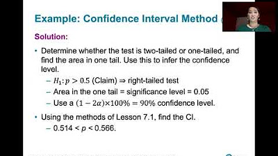
8.2.2 Testing a Claim About A Proportion - Confidence Interval Method, Comparison to Other Methods
STAT243Z 02/29/24 Zoom Recording
5.0 / 5 (0 votes)
Thanks for rating: