Demand and Inverse Demand Function | (How to find the INVERSE demand equation) | Think Econ
TLDRThis educational video clarifies the distinction between the demand equation and its inverse in economics. It begins with the standard downward-sloping demand curve, emphasizing the correct axis labeling. The script presents a linear demand equation, QD = 240 - 5P, and then demonstrates step-by-step the algebraic process of transforming it into the inverse demand function, P = 48 - 0.2Q. The video encourages viewers to practice this skill, highlighting the importance of understanding both functions for economic analysis.
Takeaways
- 📈 The video discusses the difference between the demand equation and the inverse demand equation in economics.
- 📊 It emphasizes the importance of correctly labeling axes with price on the Y-axis and quantity on the X-axis for a demand curve.
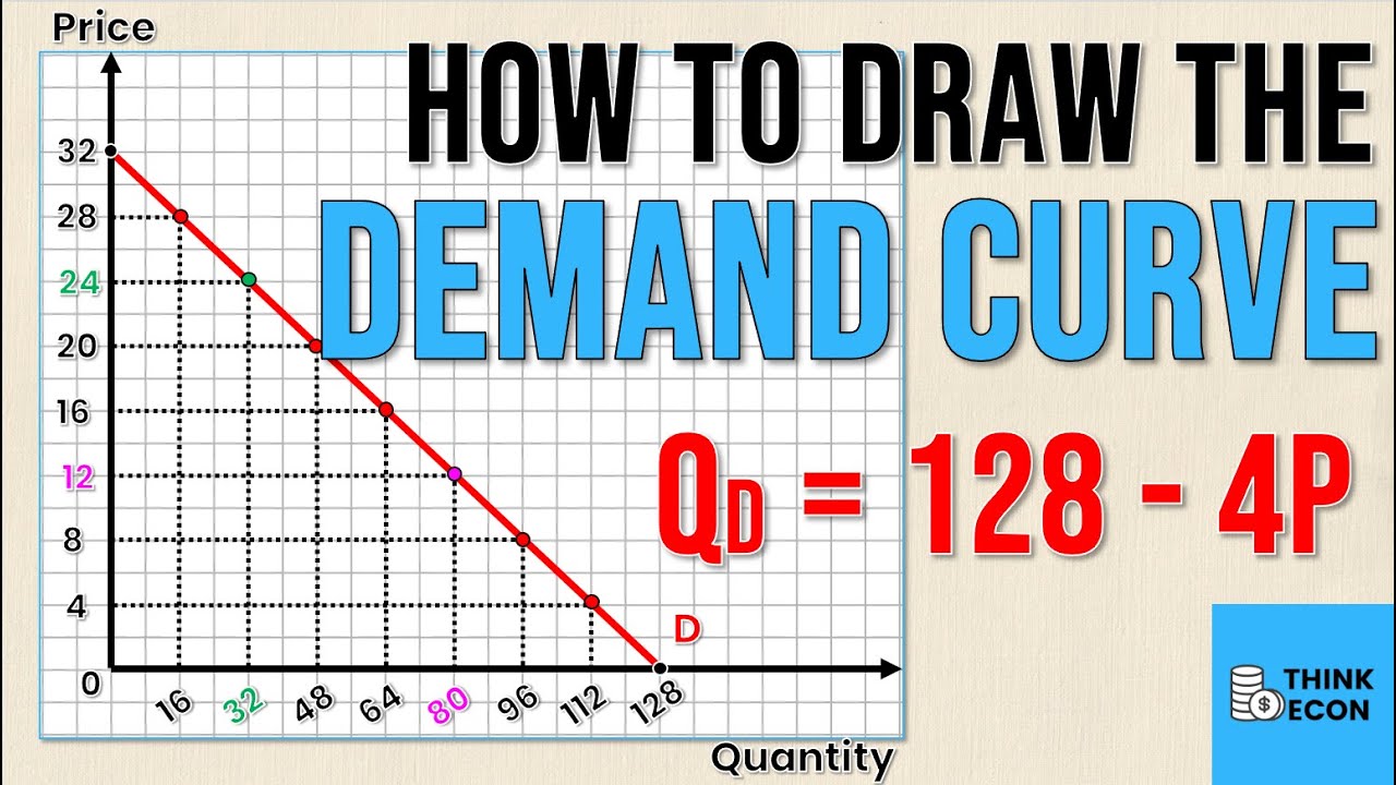
- 🔍 The script provides an example of a general demand equation, QD = 240 - 5P, illustrating the negative relationship between price and quantity demanded.
- 📚 The law of demand is mentioned, which states that there is a negative correlation between price and quantity demanded.
- ✏️ The video demonstrates how to algebraically manipulate the demand equation to derive the inverse demand function.
- 🔄 The process involves isolating P (price) and making it the dependent variable, which involves switching sides and changing signs.
- 📝 The inverse demand function is derived to be P = 48 - 0.2Q, showing price as a function of quantity demanded.
- 📉 The video explains that the inverse demand function is not just a different form but a rearrangement of the original demand equation.
- 📈 It clarifies that in economics, the demand curve typically represents the inverse demand function, even though the original equation is used for algebraic solutions.
- 📚 The script encourages viewers to practice deriving the inverse demand function from any given demand equation and vice versa.
- 👍 The video concludes by inviting viewers to engage with the channel through likes, subscriptions, and comments for future topic suggestions.
Q & A
What is the main topic of the video?
-The main topic of the video is explaining the difference between the demand equation and the inverse demand equation in economics.
Why is it important to label the axes correctly when drawing a demand curve?
-It is important to label the axes correctly because placing price on the vertical axis (y-axis) and quantity on the horizontal axis (x-axis) is a standard in economics. Mislabeling can lead to confusion and loss of marks in assessments.
What is the general form of a demand equation as presented in the video?
-The general form of the demand equation presented in the video is QD = 240 - 5P, where QD represents the quantity demanded and P represents the price.
What is the relationship between QD and P as per the law of demand?
-According to the law of demand, there is a negative relationship between QD (quantity demanded) and P (price), meaning that as price increases, the quantity demanded decreases, and vice versa.
How is the inverse demand function derived from the original demand equation?
-The inverse demand function is derived by isolating P (price) instead of QD (quantity demanded). This involves switching the sides of the equation and dividing each term by the coefficient of P.
What is the inverse demand function for the given demand equation?
-The inverse demand function for the given demand equation is P = 48 - 0.2Q, where P is the price and Q is the quantity demanded.
What does the negative coefficient on P in the demand equation signify?
-The negative coefficient on P signifies the inverse relationship between price and quantity demanded, which is consistent with the law of demand.
Why is it recommended to convert fractions to decimals in the inverse demand function if possible?
-Converting fractions to decimals in the inverse demand function is recommended because many people find it easier to work with finite decimals rather than fractions, especially in economic calculations.
What is the significance of functional notation in the context of demand and inverse demand functions?
-Functional notation, such as Q of P or P of Q, signifies the dependent variable (quantity or price) as a function of the independent variable (price or quantity), clearly indicating the relationship between the two variables.
Why is the original demand function typically used for graphing, even though the inverse demand function is also valid?
-The original demand function is typically used for graphing because it follows the standard convention of having quantity on the x-axis and price on the y-axis, which is more intuitive for visual representation in economics.
What does the video suggest for viewers who want to practice understanding demand and inverse demand functions?
-The video suggests that viewers should practice by taking the original demand function, rearranging it to find the inverse demand function, and vice versa, to solidify their understanding of the concepts.
Outlines
📚 Introduction to Demand and Inverse Demand Equations
The video script begins with a warm welcome to the channel and an introduction to the topic of the difference between the demand equation and the inverse demand equation. The speaker emphasizes the importance of correctly labeling axes in economic graphs, with price on the y-axis and quantity on the x-axis, to avoid losing marks in assessments. A general demand equation, QD = 240 - 5P, is presented to illustrate the negative relationship between quantity demanded (QD) and price (P), as per the law of demand. The script then introduces the concept of functional notation and the process of deriving the inverse demand function from the original demand equation.
Mindmap
Keywords
💡Demand Curve
💡Demand Equation
💡Inverse Demand Equation
💡Law of Demand
💡Functional Notation
💡Dependent and Independent Variables
💡Linear Equation
💡Algebraic Manipulation
💡Graphing
💡Economic Principles
💡Homework Assignment
Highlights
Introduction to the difference between the demand equation and the inverse demand equation.
Importance of correctly labeling axes with price on the Y-axis and quantity on the X-axis for the demand curve.
Explanation of the general demand equation QD = 240 - 5P, illustrating the negative relationship between price and quantity demanded.
Clarification on functional notation and the dependent and independent variables in the demand function.
Step-by-step guide on how to derive the inverse demand function from the original demand function.
Switching sides of the equation to isolate P and changing the sign of the coefficient when doing so.
Division of terms to solve for P in the inverse demand function, simplifying the equation.
Conversion of fractions to decimals for ease of use in the inverse demand function.
Final form of the inverse demand function P = 48 - 0.2QD, with functional notation P(Q) = 48 - 0.2Q.
Graphical representation of the demand curve and the inverse demand function on a graph.
Discussion on the general form of a linear equation and its application to the inverse demand function.
Misunderstanding often seen in economics regarding the graphing of the inverse demand function instead of the original.
Advice on practicing the algebraic manipulation of demand functions for better understanding.
Invitation for viewers to engage with the channel by liking, subscribing, and commenting on the video.
Encouragement for viewers to suggest economic topics or homework questions for future video content.
Closing remarks and sign-off for the video, promising to see viewers in the next video.
Transcripts
Browse More Related Video
5.0 / 5 (0 votes)
Thanks for rating:


