Managerial Economics 4.3: Cost Minimization
TLDRThe video script presents a detailed exploration of cost minimization in managerial economics. It introduces the concept of the isocost line, which represents combinations of capital and labor that yield the same total cost. The script explains how to calculate the slope of the isocost line and uses an example with given wage and rental rates to illustrate the graphical representation of isocosts. The cost minimization process is then discussed, aiming to achieve a target output with the least expenditure on inputs. This involves comparing the marginal product per dollar for labor and capital to determine the optimal mix of these inputs. The script also covers three different production functions: Cobb-Douglas, Leontief, and Linear, explaining how to apply cost minimization principles to each. The video concludes with a graphical illustration of the cost minimization process, showing how the isocost line becomes tangent to the isoquant at the optimal point, aligning with the principles of utility maximization.
Takeaways
- 📈 **Cost Minimization**: The goal is to produce a target output with the least amount of cost on inputs, similar to the consumer's problem of maximizing utility.
- 📊 **Isocost Line**: An isocost line represents combinations of capital and labor that have the same total cost, with the equation C = wL + rK, where w is the wage and r is the rental rate of capital.
- 💲 **Slope of Isocost**: The slope of the isocost line is given by w/r, which is the ratio of the price of labor to the price of capital.
- 📉 **Graphical Isocost**: Isocost lines are straight and downward sloping, and there is an infinite number corresponding to any possible total cost C.
- ✍️ **Marginal Product per Dollar**: To minimize cost, compare the marginal product per dollar for labor (MPL/W) and capital (MPK/r), adjusting the mix of inputs accordingly.
- 🔑 **Cost Minimization Condition**: The condition for cost minimization is MPL/W = MPK/r, which means the marginal rate of technical substitution equals the ratio of input prices.
- 🔍 **Tangency Condition**: The isocost line should be tangent to the isoquant corresponding to the target output, indicating the cost-minimizing combination of labor and capital.
- 🔢 **Cobb-Douglas Production Function**: For this function, cost minimization involves setting the marginal rate of technical substitution equal to the ratio of input prices and solving a system of equations.
- 🔄 **Leontief Production Function**: In the case of Leontief production functions, cost minimization requires that aK = bL = Q, ensuring no input is wasted.
- 🔩 **Linear Production Function**: For linear functions, there are three cases for input use: all labor if MPL/W > MPK/r, all capital if MPL/W < MPK/r, or any combination if MPL/W = MPK/r.
- 📐 **Graphical Approach**: The graphical approach to cost minimization involves finding the point where the isocost is tangent to the isoquant, which is the most cost-efficient combination of inputs.
Q & A
What is the concept of an isocost line in the context of managerial economics?
-An isocost line represents combinations of capital and labor that have the same total cost. It is a graphical tool used to analyze the cost minimization for a given level of output, assuming the prices of labor (w) and capital (r) are constant.
How is the total cost (C) calculated in terms of labor (L) and capital (K)?
-The total cost (C) is calculated as the sum of the cost of labor and the cost of capital, which is expressed as C = wL + rK, where w is the wage (price of a unit of labor) and r is the rental rate (price of a unit of capital).
What does the slope of the isocost line represent?
-The slope of the isocost line represents the ratio of the price of labor to the price of capital (w/r). It indicates how much capital can be substituted for labor, or vice versa, without changing the total cost.
How do you find the intercepts of an isocost line when graphing?
-To find the intercepts of an isocost line, you set one of the variables to zero and solve for the other. For the labor (L) intercept, set K=0 and solve for L. For the capital (K) intercept, set L=0 and solve for K.
What is the primary goal of cost minimization?
-The primary goal of cost minimization is to attain a certain target output while spending as little as possible on inputs, similar to the consumer's problem of maximizing utility but focusing on minimizing costs.
What is the condition for cost minimization in terms of the marginal product of labor (MPL) and the marginal product of capital (MPK)?
-The condition for cost minimization is that the marginal product per dollar for labor (MPL/W) should equal the marginal product per dollar for capital (MPK/R). If MPL/W > MPK/R, use more labor; if MPL/W < MPK/R, use more capital; if they are equal, the cost is minimized.
What does the marginal rate of technical substitution (MRTS) represent in the context of cost minimization?
-The MRTS represents the rate at which one input can be substituted for another while keeping the output constant. At the point of cost minimization, the MRTS should be equal to the ratio of the input prices (w/r).
How does the shape of the isoquant for the Cobb-Douglas production function facilitate cost minimization?
-The curved shape of the Cobb-Douglas isoquants allows for the traditional method of cost minimization, where the isocost line is tangent to the isoquant. This tangency point represents the optimal mix of labor and capital that minimizes cost for a given level of output.
What are the three possible cases for the ratio of MPL/W to MPK/R in the context of a linear production function?
-The three possible cases are: 1) MPL/W > MPK/R, where it's more cost-effective to use more labor; 2) MPL/W < MPK/R, where it's more cost-effective to use more capital; and 3) MPL/W = MPK/R, where any combination of labor and capital that produces the required output is equally cost-effective.
How does the Leontief production function differ from the Cobb-Douglas and linear production functions in terms of cost minimization?
-The Leontief production function differs by having L-shaped isoquants, which means that the cost-minimizing point is always at the corner of the L, indicating that the firm will use either all labor or all capital to produce the output, but not a mix of both.
What is the graphical representation of the cost minimization process for a firm?
-The graphical representation involves plotting the isocost line and the isoquant corresponding to the target output on the same graph. The firm seeks the point where the isocost line is tangent to the isoquant, indicating the optimal combination of labor and capital that minimizes the cost for producing the desired output.
Outlines
📊 Introduction to Cost Minimization and Isocost
Sebastian Y introduces the concept of cost minimization in managerial economics. He begins by defining key parameters such as the wage (w) for labor and the rental rate (r) for capital, assuming these are constant. An isocost line is then explained as a combination of capital (k) and labor (l) that maintain the same total cost (c), which equals w*l + r*k. The slope of the isocost line is w/r, the ratio of the prices of labor and capital. An example is given with w=2 and r=8, and the isocost equations for total costs of 160 and 200 are derived and graphed. The concept of tangency between the isocost and the isoquant at the point of cost minimization is introduced, which is akin to the tangency between a budget line and an indifference curve in consumer theory.
🔍 Cost Minimization Conditions and Cobb-Douglas Production Function
The video continues with the conditions for cost minimization, emphasizing the marginal product per dollar for labor (MPL/W) and capital (MPK/R). It is stated that if MPL/W > MPK/R, more labor should be used, and vice versa. The condition for minimized cost is MPL/MPK = W/R, which is derived algebraically. This is related to the marginal rate of technical substitution (MRTS) and the ratio of input prices. The process of finding the cost-minimizing point involves the isocost being tangent to the isoquant. The Cobb-Douglas production function is used as an example to illustrate this process. The function f(k, l) = k^a * l^b is given, and cost minimization is demonstrated by setting MRTS equal to the ratio of input prices and solving for the optimal combination of k and l for a target output q.
📈 Linear Production Function and Cost Minimization
The linear production function f(k, l) = a*k + b*l is discussed, and the marginal product of labor per dollar (MPL/W) and the marginal product of capital per dollar (MPK/R) are calculated. It is noted that with a linear function, there are three cases: MPL/W > MPK/R (use more labor), MPL/W < MPK/R (use more capital), and MPL/W = MPK/R (any mix of labor and capital is optimal). An example is provided with the function f(k, l) = 3*k + 2*l, a wage of 4, a rental rate of 8, and a target output of 60. The calculations show that labor is the better value, leading to an all-labor, no-capital solution with 30 units of labor and a total cost of 120. The graph illustrates the isoquant and isocost as straight lines, with the isocost being flatter than the isoquant, indicating all labor is used.
🔗 Leontief Production Function and Cost Minimization
The Leontief production function, characterized by the minimum of a*k and b*l, is explored. The cost minimization process for this function is straightforward, requiring that a*k = b*l = q, ensuring no waste of inputs. The isocosts for the Leontief function are L-shaped, and the cost-minimizing point is at the corner of the L. An example with the function f(k, l) = min(k, 0.5*l), a wage of 4, a rental rate of 2, and a target output of 20 is provided. The calculations yield 20 units of capital and 40 units of labor, with a total cost of 200. The graph shows the cost-minimizing point, the L-shaped isoquant, and the isocost, demonstrating that the isocost touches the isoquant at the corner, which is the optimal point.
📉 Summary of Cost Minimization Across Production Functions
The video concludes with a summary of how to minimize costs across three different production functions. It emphasizes the similarities between cost minimization and utility maximization in consumer theory, highlighting the importance of tangency between the isocost and the isoquant. The process for each production function is reviewed, and it is noted that in the next video, further discussion on cost will take place, providing a comprehensive understanding of cost minimization in managerial economics.
Mindmap
Keywords
💡Cost Minimization
💡Isocost
💡Wage (w)
💡Rental Rate (r)
💡Isoquant
💡Marginal Product per Dollar (MPL/W and MPK/R)
💡Cobb-Douglas Production Function
💡Linear Production Function
💡Leontief Production Function
💡Target Output (Q)
💡Total Cost (C)
Highlights
Introduction to cost minimization in managerial economics
Definition of wage (w) as the price of a unit of labor and rental rate (r) as the price of a unit of capital
Assumption of constant w and r, implying no overtime pay or similar variables
Explanation of isocost as a line containing combinations of capital and labor with the same total cost
Total cost (C) formula: C = w*l + r*k where l is labor and k is capital
Graphical representation and calculation of isocost intercepts for given cost (C) values
Slope of the isocost is the ratio of the prices (w/r), which is crucial for cost minimization
Cost minimization involves attaining a target output with minimal input expenditure
Marginal product per dollar for labor (MPL/W) and capital (MPK/R) as decision-making metrics
Condition for cost minimization: MPL/W = MPK/R, leading to the optimal input mix
MRTS (Marginal Rate of Technical Substitution) equals the ratio of input prices (w/r)
Cost minimization graphically represented as the tangency of isocost and isoquant
Cobb-Douglas production function example with cost minimization calculation
Linear production function and its cost minimization approach with constant MPL/W and MPK/R
Three possible cases for linear production function based on the relationship between MPL/W and MPK/R
Leontief production function's cost minimization method and its L-shaped isoquants
Example calculation and graphical representation for Leontief production function
Summary of cost minimization for three production functions: Cobb-Douglas, Linear, and Leontief
Transcripts
Browse More Related Video
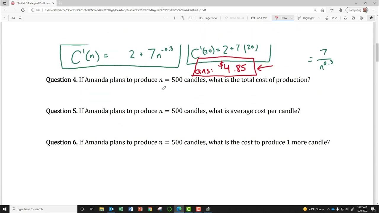
BusCalc 10 Marginal Profit
Business Calculus - Math 1329 - Section 7.1 - Functions of Several Variables
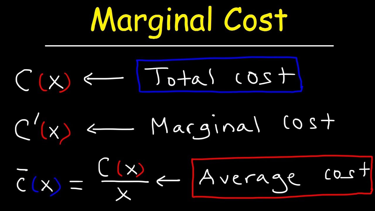
Marginal Cost and Average Total Cost

Marginal Revenue, Average Cost, Profit, Price & Demand Function - Calculus
Business Calculus - Math 1329 - Section 1.3 - Lines and Linear Functions
Marginal and Average Cost
5.0 / 5 (0 votes)
Thanks for rating: