Worked example: Logistic model word problem | Differential equations | AP Calculus BC | Khan Academy
TLDRThe video script presents a detailed exploration of the logistic differential equation, a mathematical model often used to describe population growth under environmental constraints. It explains that the rate of population change is proportional to the product of the current population and the difference between a carrying capacity and the current population. The carrying capacity, in this case, is identified as 48,000 bacteria, representing the maximum population size the environment can sustain indefinitely. The script also addresses the question of when the population grows the fastest, which is found to be at half the carrying capacity, or 24,000 bacteria. The explanation uses both algebraic manipulation and graphical representation to convey the concepts clearly, ultimately demystifying the logistic differential equation and its practical implications for population dynamics.
Takeaways
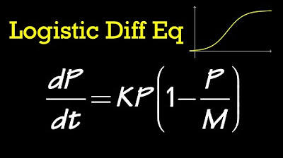
- 🌿 **Logistic Differential Equation**: The rate of change of a population (P) with respect to time (T) is proportional to the product of the population and the difference between the carrying capacity (A) and the population itself.
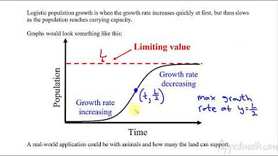
- 📈 **Population Growth**: When the population is small, the environment isn't a limiting factor, leading to an accelerating growth rate that slows as the population approaches the carrying capacity.
- 🐰 **Environmental Limitations**: As the population grows, environmental factors will eventually limit further growth, causing the rate of change to decrease as the population nears the carrying capacity.
- 📊 **Typical Logistic Graph**: The logistic model is often represented graphically, showing an S-shaped curve where growth accelerates from a small population and then decelerates as it approaches the carrying capacity.
- ∞ **Carrying Capacity**: The carrying capacity (A) is the maximum population size that the environment can sustain indefinitely, which the logistic model approaches as time (T) goes to infinity.
- 🔍 **Finding the Carrying Capacity**: The carrying capacity can be identified by setting the derivative of the logistic equation to zero and solving for the population (P), which in this case is 48,000 bacteria.
- 📌 **Maximum Growth Rate**: The population grows the fastest when it is halfway between zero and the carrying capacity, which can be found by analyzing the logistic equation as a quadratic function of P.
- ⏳ **Approaching Equilibrium**: As time progresses, the rate of population change decreases and the population size asymptotically approaches the carrying capacity.
- 🔢 **Quadratic Analysis**: The logistic differential equation can be rewritten in a form that highlights it as a quadratic function, where the vertex of the parabola represents the population size at the maximum growth rate.
- 📐 **Vertex of the Parabola**: The vertex of the downward-opening parabola, representing the maximum growth rate, is found at half the carrying capacity when the population is at 24,000 bacteria.
- 🧮 **Calculus and Algebra Tools**: Both calculus and algebra can be used to identify the maximum growth point of the population, which is essentially the vertex of the logistic growth curve.
Q & A
What is the logistic differential equation?
-The logistic differential equation is a mathematical model that describes the growth of a population over time, where the growth rate is proportional to the population size and the difference between the population size and the carrying capacity.
What is the carrying capacity in the context of the logistic differential equation?
-The carrying capacity is the maximum population size that the environment can sustain indefinitely. It is a constant in the logistic differential equation that represents the limit of population growth.
How is the rate of population change related to the population size and carrying capacity in the logistic model?
-In the logistic model, the rate of population change is proportional to the product of the current population size and the difference between the carrying capacity and the current population size.
What happens to the rate of population change as the population size approaches zero?
-As the population size approaches zero, the rate of population change also approaches zero, since there would be no individuals to reproduce and increase the population.
How does the logistic model account for environmental limitations on population growth?
-The logistic model accounts for environmental limitations by including a carrying capacity. As the population size approaches the carrying capacity, the rate of population change decreases, eventually approaching zero, thus limiting the population growth.
What is the carrying capacity of the bacteria population in the given logistic differential equation?
-The carrying capacity of the bacteria population in the given logistic differential equation is 48,000 bacteria.
At what population size is the bacteria population growing the fastest?
-The bacteria population is growing the fastest at a population size of 24,000, which is halfway between the carrying capacity and zero.
What is the significance of the quadratic expression in the logistic differential equation?
-The quadratic expression in the logistic differential equation represents the rate of change of the population as a function of the population size. It is a concave downward parabola, indicating that the rate of change increases with population size until it reaches a maximum and then decreases as the population approaches the carrying capacity.
How can you determine the maximum growth rate of the population in the logistic model?
-The maximum growth rate of the population in the logistic model can be determined by finding the vertex of the concave downward parabola represented by the quadratic expression. This occurs at a population size halfway between the carrying capacity and zero.
Why is the logistic model useful for studying population dynamics?
-The logistic model is useful for studying population dynamics because it accounts for the initial exponential growth of a population when it is small and the subsequent slowing of growth as the population size approaches the carrying capacity, reflecting real-world environmental limitations.
What is the initial population size of the bacteria in the given problem?
-The initial population size of the bacteria in the given problem is 700 bacteria.
How does the logistic model differ from a simple exponential growth model?
-The logistic model differs from a simple exponential growth model by incorporating a carrying capacity, which limits the growth rate as the population size increases. In contrast, an exponential growth model assumes that the growth rate remains constant, leading to unlimited population growth.
Outlines
📚 Introduction to Logistic Differential Equation
The first paragraph introduces the logistic differential equation, which models population growth with a carrying capacity. The narrator explains that the rate of population change is proportional to the population and the difference between the carrying capacity and the current population. As the population nears the carrying capacity, the growth rate slows down. The carrying capacity is identified as the population size when the growth rate approaches zero over time. The logistic equation is manipulated to its standard form to reveal that the carrying capacity is 48,000 bacteria.
🔍 Finding the Maximum Growth Rate
The second paragraph delves into determining the population size at which the growth rate is the fastest. It is explained that the rate of change is initially small when the population is low and increases until it reaches a peak before declining as the population approaches the carrying capacity. The logistic differential equation is identified as a quadratic function of the population, which is concave downward. The maximum growth rate occurs at half the distance between the carrying capacity (48,000) and zero. Using calculus and algebra, the vertex of the parabola is found to be at a population size of 24,000, indicating this is when the population grows the fastest.
Mindmap
Keywords
💡Logistic Differential Equation
💡Carrying Capacity
💡Rate of Change
💡Initial Population
💡Environment Limitation
💡Quadratic Expression
💡Maximum Rate of Change
💡Vertex
💡Zero Growth Point
💡Time (T)
💡Population Size (P)
Highlights
The logistic differential equation models the rate of change of a population over time, with respect to the population size and carrying capacity.
When the population is small, the environment is not a limiting factor and the population grows exponentially.
As the population approaches the carrying capacity, the rate of growth slows down and eventually approaches zero.
The logistic equation can be written in the form dP/dt = r * P * (A - P), where r is the growth rate, P is the population, and A is the carrying capacity.
The carrying capacity (A) is the maximum population size that the environment can sustain indefinitely.
In the given problem, the carrying capacity is 48,000 bacteria, as the population approaches this value when time goes to infinity.
The population grows the fastest when it is halfway between its initial size and the carrying capacity.
The maximum growth rate occurs at a population size of 24,000, which is halfway between 0 and the carrying capacity of 48,000.
The logistic equation can be viewed as a quadratic function of population size, with a downward-opening parabola shape.
The maximum growth rate corresponds to the vertex of the parabola, which is halfway between the x-intercepts (population size of 0 and carrying capacity).
The logistic model is useful for studying population dynamics, especially in situations where the environment imposes a limit on population growth.
The model assumes that the population starts from a non-zero value, as a population of zero would not grow.
The rate of population change increases as the population grows, until it reaches a maximum and then starts to decrease as the carrying capacity is approached.
The logistic equation can be solved and analyzed using calculus and algebraic techniques to find the carrying capacity and maximum growth rate.
Recognizing the logistic equation and understanding the relationship between population size, growth rate, and carrying capacity is key to solving and interpreting the model.
The logistic model can be intimidating at first, but breaking it down into components and using graphical and mathematical tools makes it more approachable.
The model provides insights into how population growth is influenced by environmental factors and how it approaches a stable equilibrium over time.
Transcripts
Browse More Related Video
Logistic Differential Equation (general solution)
Solving the logistic differential equation part 2 | Khan Academy
The Logistic Equation and the Analytic Solution
Calculus BC – 7.9 Logistic Models with Differential Equations
Logistic growth versus exponential growth | Ecology | AP Biology | Khan Academy
Logistic Growth
5.0 / 5 (0 votes)
Thanks for rating: