Regression diagnostics and analysis workflow
TLDRThis video outlines a comprehensive workflow for conducting regression analysis, emphasizing the importance of hypothesis formulation, data exploration, and model estimation. It highlights the use of diagnostic plots over statistical tests for assumptions checking, such as linearity, independence of observations, and homoscedasticity. The video demonstrates the process using the Prestige dataset, discussing the interpretation of residuals and the identification of outliers. It suggests potential model improvements, like considering heteroscedasticity robust standard errors and log transformation of income, to enhance the analysis.
Takeaways
- 📝 The video outlines a workflow for conducting regression analysis, emphasizing the importance of hypothesis testing, data collection, and model diagnostics.
- 🔍 The process begins with stating a hypothesis, collecting data, exploring relationships, estimating the initial regression model, and performing diagnostics.
- 📊 The speaker prefers using plots over statistical tests for diagnostics as they provide more insight into the nature of potential problems.
- 🔎 The diagnostic process involves checking the six regression assumptions, such as linearity, independence of observations, no perfect collinearity, and assumptions about the error term.
- 📈 The speaker uses the Prestige dataset to demonstrate the regression analysis diagnostics, focusing on the ordinary least squares (OLS) assumptions checking.
- 📚 The assumptions about the error term include having an expected value of zero, equal variance (homoscedasticity), and being normally distributed.
- 📊 Residuals are used as estimates of the error term, and analyzing them is central to regression diagnostics.
- 🎯 The normal Q-Q plot is used to check the normality of residuals and can help identify outliers.
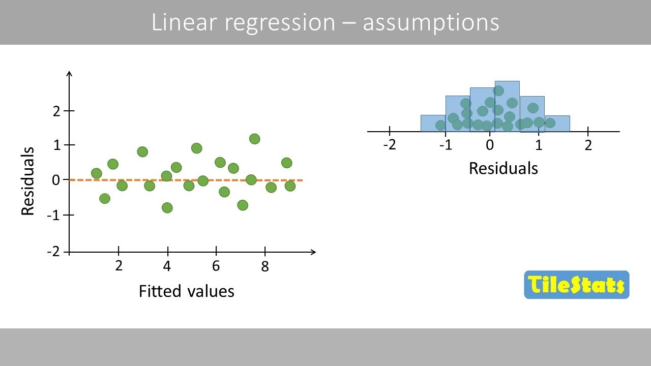
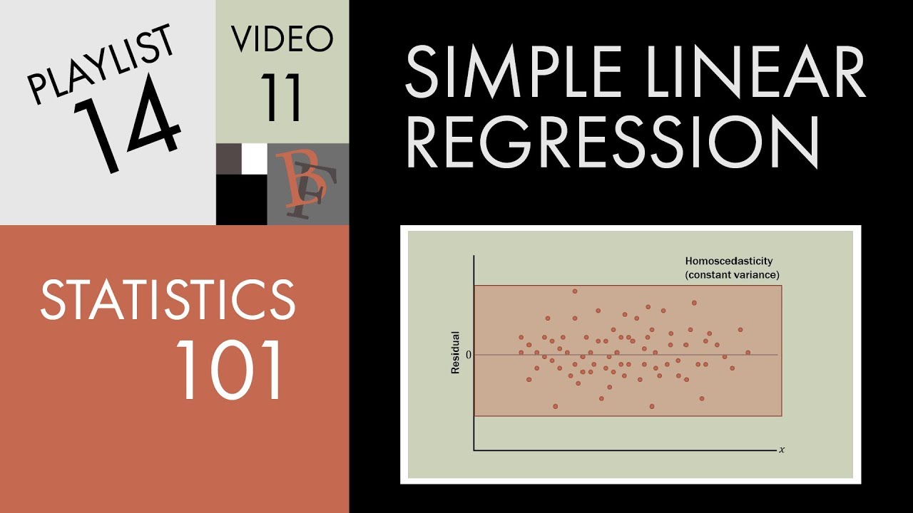
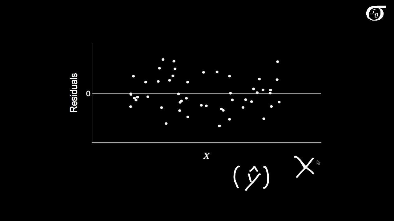
- 📉 The residual vs. fitted plot is used to test for nonlinearities and heteroscedasticity, looking for patterns that might indicate issues with the model fit.
- 🚫 The presence of heteroscedasticity in the data suggests that the error term's variance is not constant, which may require the use of robust standard errors or model adjustments.
- 🔍 Identifying outliers involves examining plots such as the residual vs. leverage plot and considering Cook's distance to determine influential observations.
- 🛠️ After diagnostics, the model may be refined by considering transformations (e.g., log transformation for income), dropping influential observations, or using robust standard errors.
Q & A
What is the main focus of the video?
-The video focuses on demonstrating a possible workflow for conducting regression analysis, including the steps for hypothesis testing, data exploration, model estimation, diagnostics, and interpretation of results.
Why is it important to understand the relationships in the data during the data exploration phase?
-Understanding the relationships in the data is crucial as it helps in forming a clear hypothesis and guides the selection of appropriate statistical models and variables for the regression analysis.
What does the speaker prefer to use over statistical tests when conducting diagnostics in regression analysis?
-The speaker prefers using plots over statistical tests because plots can provide a more informative visual representation of the data, helping to identify the nature of potential problems more effectively.
What are the six assumptions of regression analysis mentioned in the video?
-The six assumptions are: 1) linear relationships, 2) independence of observations, 3) no perfect collinearity and non-zero variances of independent variables, 4) error term has an expected value of zero, 5) error term has equal variance (homoscedasticity), and 6) error term is normally distributed.
How does the speaker suggest identifying the nature of heteroscedasticity problems?
-The speaker suggests looking at the actual distribution of the residuals rather than relying solely on statistical tests. By examining the residuals, one can better understand the nature of the heteroscedasticity issue.
What is the purpose of the normal Q-Q plot in regression diagnostics?
-The normal Q-Q plot is used to quantify whether the regression residuals are normally distributed. It provides a visual comparison between the residuals and the normal distribution, helping to identify any significant deviations.
What does the residual vs. fitted plot help to identify?
-The residual vs. fitted plot helps to test for nonlinearities and heteroscedasticity in the data. It allows us to see if there are any patterns in the residuals that might indicate issues with the model's fit.
How can the influence of outliers be determined using the residual versus leverage plot?
-The residual versus leverage plot helps identify observations that have both high leverage and high residual values. These observations may be influential and could potentially skew the results of the regression analysis.
What is the added-variable plot, and what does it measure?
-The added-variable plot quantifies the relationship between the dependent variable and one independent variable at a time, while controlling for the effects of other independent variables. It helps to identify nonlinearities and heteroscedasticity in a more refined manner.
What are some potential modifications to the model suggested after conducting diagnostics?
-Some potential modifications include using heteroscedasticity robust standard errors, dropping outliers like general managers, considering log transformation of income, and re-estimating the model with and without certain outlier observations to perform a robustness check.
Why might log transformation of income be considered in the model?
-Log transformation of income can be considered because it makes more sense to view income in relative terms. This transformation helps to normalize the data and better capture the percentage increase in income, which is typically more meaningful in the context of salary negotiations and quality of life improvements.
Outlines
📊 Comprehensive Regression Analysis Workflow
The video introduces a detailed workflow for conducting regression analysis, emphasizing the empirical testing of assumptions inherent in the process. The presenter opts for R as the primary tool, acknowledging that Stata and SPSS are viable alternatives. The workflow begins with hypothesis formulation, followed by data collection and exploration to understand variable relationships. The initial regression model involves identifying dependent and independent variables, then briefly reviewing the results. The focus shifts to diagnostics, favoring plots over statistical tests for a more nuanced understanding of issues like heteroscedasticity, rather than merely confirming their presence. The presenter iteratively refines the regression model by addressing identified problems such as non-linear relationships, outliers, or heteroscedasticity, until a satisfactory model is achieved. This model is then subjected to nested model tests against alternatives. Finally, the presenter emphasizes the importance of interpreting regression coefficients within the research context, using the Prestige dataset as an example to explore education, income, and gender distribution as factors influencing occupational prestige.
🔍 Diagnosing Regression Models Using Residuals
This segment delves into the diagnostics phase of regression analysis, highlighting the critical role of residuals—differences between observed and predicted values—as estimates of error terms. The presenter begins with the normal Q-Q plot to assess the normality of residuals, indicating a well-fitting model if residuals are normally distributed. This step also helps identify outliers and potential issues with the model. The discussion then moves to the residual vs. fitted plot, which is used to detect non-linear relationships and heteroscedasticity. The presenter describes various patterns that might emerge in this plot, such as a 'butterfly shape' indicating heteroscedasticity or a 'megaphone' shape suggesting both nonlinearity and heteroscedasticity. The aim is to observe a pattern-free distribution of residuals against fitted values, signaling a well-fitting model.
📈 Advanced Diagnostics and Dealing with Outliers
This part continues the exploration of regression diagnostics, focusing on further scrutiny of the variance of estimates and the presence of outliers. The presenter uses residual vs. leverage plots to identify influential observations, leveraging Cook's distance as a measure of an observation's influence. Specific professions are examined for their prestigiousness relative to the model's predictions, revealing instances where the model may significantly over or under-predict. This section suggests potential responses to identified issues, such as considering heteroscedasticity robust standard errors or modifying the data (e.g., removing outliers) to refine the model. The emphasis is on applying judgment and domain knowledge to interpret and act upon diagnostic findings.
🔬 Refining Regression Models Through Transformation and Analysis
The final segment discusses the steps following diagnostics, focusing on adjusting the regression model to address identified issues. The presenter suggests practical interventions, like using heteroscedasticity robust standard errors or considering the removal of influential observations (e.g., 'general managers') to check the robustness of the model. Additionally, the importance of log transformation for variables like income is highlighted to account for the relative significance of changes in such variables. The video underscores that these adjustments, informed by diagnostic plots and tests, are crucial for refining the regression model to better reflect the underlying data and research questions.
Mindmap
Keywords
💡Regression Analysis
💡Assumptions
💡Diagnostics
💡Residuals
💡Heteroscedasticity
💡Nonlinear Relationships
💡Outliers
💡Standard Errors
💡Transformation
💡Cook's Distance
💡Added-variable Plot
Highlights
The video outlines a workflow for conducting regression analysis, emphasizing the importance of testing assumptions and using diagnostics.
Regression analysis begins with stating a hypothesis and collecting data, followed by data exploration and model estimation.
The speaker prefers using plots over statistical tests for diagnostics because plots provide more information about the nature of the problem.
The first regression model is estimated with independent and dependent variables, and the results are briefly checked.
Diagnostics involve various plots, and the speaker identifies the biggest problem before refining the model.
Nested model tests are conducted against alternative models after finalizing the model through diagnostics.
Interpreting the regression coefficients in the context of the research is crucial for understanding their significance.
The Prestige dataset is used for demonstration, with prestige as the dependent variable and education, income, and share of women as independent variables.
Regression assumptions are checked using the OLS method, with six key assumptions outlined.
The fourth assumption states that the error term has an expected value of zero given any values of independent variables.
The fifth assumption is the homoscedasticity assumption, which requires the error term to have equal variance.
The sixth assumption is that the error term is normally distributed, which is tested using the normal Q-Q plot of residuals.
The residual vs. fitted plot is used to test for nonlinearities and heteroscedasticity in the data.
The influence plot or outlier plot helps identify influential observations with high leverage and large residuals.
The added-variable plot quantifies the relationship between the dependent variable and one independent variable at a time, accounting for other variables.
The video suggests considering heteroscedasticity robust standard errors, dropping outliers, and log transformation of income as potential model refinements.
The speaker emphasizes the importance of using judgment when deciding whether to drop outliers and the impact of such decisions on the sample size.
Transcripts
Browse More Related Video

Checking Linear Regression Assumptions in R | R Tutorial 5.2 | MarinStatsLectures
Assumptions in Linear Regression - explained | residual analysis
Statistics 101: Linear Regression, Residual Analysis

interpreting residual graphs
10.2.6 Regression - Residual Plots and Their Interpretation
Simple Linear Regression: Checking Assumptions with Residual Plots
5.0 / 5 (0 votes)
Thanks for rating: