8.5 ODE Algorithms
TLDRThis video script delves into the world of ordinary differential equations, focusing on their standard form and algorithms for solving them. It reviews forced oscillations, introduces time stepping and leapfrogging techniques, and discusses Euler's method and the more advanced Runge-Kutta methods. The script emphasizes the importance of accurate algorithms for scientific predictions, such as those used in global warming models, and guides viewers through the process of applying these methods to physical problems like spring-mass systems.
Takeaways
- 📚 The lecture continues the exploration of ordinary differential equations (ODEs), focusing on applying algorithms to solve them.
- 🔍 The importance of having ODEs in a standard form is emphasized for consistency and ease of application of algorithms.
- 🌟 The script reviews forced oscillations, a physical problem involving a mass attached to a spring with an external driving force, represented by Newton's second law.
- 📉 The standard form of an ODE is presented as a first-order derivative, with the equation detailed in the script.
- 🔑 The concept of 'leapfrogging' or 'time stepping' is introduced as a method to solve ODEs by advancing the solution in small steps.
- 🔄 The script explains that the accuracy of the leapfrogging method improves with smaller time steps, but a balance is needed to avoid excessive computation due to round-off errors.
- 📐 Euler's method, a simple first-order algorithm, is discussed for its ease of use and its role as a starting point for more sophisticated methods.
- 📈 Runge-Kutta methods are introduced as higher-order algorithms that provide more precise solutions than Euler's method, with a focus on the second-order (RK2) and fourth-order (RK4) methods.
- 🔍 The script explains the process of applying the Runge-Kutta second-order method (RK2) to a spring-mass system, highlighting the improved accuracy over Euler's method.
- 🛠️ The Runge-Kutta fourth-order method (RK4) is recommended for its balance of precision and simplicity, and it's suggested that beginners use pre-existing implementations to avoid errors.
- 🔧 The script concludes by encouraging students to apply the discussed algorithms to real problems, indicating the practicality of the methods taught.
Q & A
What is the main focus of the lecture?
-The main focus of the lecture is on ordinary differential equations, specifically the development of algorithms for solving them and applying these algorithms to physical problems such as forced oscillations.
Why is having a standard form for differential equations important?
-Having a standard form for differential equations is important because it allows for the application of consistent algorithms to solve a variety of problems, making the process more systematic and efficient.
What is the significance of reviewing the standard form of differential equations?
-Reviewing the standard form of differential equations is significant because it refreshes the understanding of the structure that all differential equations are put into, which is essential for applying the algorithms correctly.
What is the physical problem being discussed in the script?
-The physical problem being discussed is forced oscillations, where a mass attached to a spring is subjected to an external driving force, resulting in a time-dependent motion.
How is Newton's second law applied in this context?
-Newton's second law is applied by formulating the problem of forced oscillations into a second-order ordinary differential equation, which is then put into standard form for solving.
What is the leapfrog technique or time stepping in the context of solving differential equations?
-The leapfrog technique, or time stepping, is a method used to solve differential equations by advancing the solution in small, uniform steps from an initial time to a final time, effectively performing a step-by-step integration.
Why is it necessary to have a complete set of initial conditions to solve a differential equation?
-A complete set of initial conditions is necessary because they provide the starting point for the solution, which is then carried forward in time using the algorithms developed for solving the differential equations.
What is Euler's rule or Euler's algorithm in the context of solving differential equations?
-Euler's rule is a simple algorithm for solving differential equations by approximating the solution at the next time step using the derivative function evaluated at the current time step and a small time step size.
What is the main idea behind the Runge-Kutta algorithms?
-The main idea behind the Runge-Kutta algorithms is to approximate the solution of a differential equation by evaluating the derivative function at multiple points within the time step and using these evaluations to improve the accuracy of the solution.
Why is it recommended to use a higher-order algorithm like Runge-Kutta 4 (RK4) for solving differential equations?
-It is recommended to use a higher-order algorithm like RK4 because it provides a better balance between accuracy and simplicity. It is very precise and works well for a wide range of problems, making it a standard choice for solving differential equations.
How does the error in Euler's algorithm compare to the error in the Runge-Kutta algorithm?
-The error in Euler's algorithm goes like h squared, meaning it is less accurate for larger step sizes. In contrast, the Runge-Kutta algorithm has an error that goes like h to the fourth power, making it more accurate even when using larger step sizes.
What is the purpose of using both superscripts and subscripts in the script when discussing the components of the solution?
-Superscripts are used to indicate different components of the solution, such as position and velocity, while subscripts are used to denote different time steps. This notation helps to clearly distinguish between the various elements of the solution process.
What is the role of the derivative function f in the standard form of a differential equation?
-The derivative function f in the standard form of a differential equation represents the rate of change of the solution with respect to time. It is a key component that needs to be known to solve the differential equation using various algorithms.
How does the accuracy of the leapfrog technique or time stepping method relate to the size of the time step h?
-The accuracy of the leapfrog technique is directly related to the size of the time step h. Keeping h small improves the accuracy of the method, but making h too small can lead to increased computational effort and potential round-off errors.
What is the significance of the term 'rule of thumb' mentioned in the script?
-The term 'rule of thumb' is used to suggest a general guideline or principle based on experience rather than theory. In the context of the script, it refers to the suggestion of having at least a hundred time steps in a typical time scale for good accuracy when solving differential equations.
Outlines
📚 Introduction to Solving Differential Equations
The speaker welcomes the audience back and outlines the session's focus on ordinary differential equations (ODEs), emphasizing the importance of having a standard form for these equations. They mention that the session will review previous material, develop algorithms for solving ODEs, and apply these tools to solve a variety of problems. The speaker also draws a parallel between the integration process in solving ODEs and the differentiation process previously discussed, suggesting that the techniques used will be familiar.
🌟 Review of Forced Oscillations and Standard Form
The speaker reviews forced oscillations, a physical problem involving a mass attached to a spring with an external driving force. They introduce Newton's second law, leading to a second-order ODE, and explain how to transform it into a standard form suitable for algorithmic solutions. The standard form is expressed as a system of first-order differential equations, with the position and velocity defined as components of a vector. The speaker also discusses the force function necessary for solving the equation.
🕒 Time Stepping and Leapfrogging Technique
The speaker introduces the concept of time stepping, or leapfrogging, a method for solving differential equations by advancing the solution in small, uniform steps. This technique is likened to building a castle on sand, as it relies on initial conditions and extrapolates them over time. The speaker discusses the importance of choosing an appropriate time step size, h, for accuracy, and touches on the challenges of long-term predictions, using global warming as an example of complex problem-solving requiring differential equations.
📉 Euler's Method and Its Limitations
The speaker presents Euler's method, a simple yet widely used algorithm for solving differential equations. They explain that the method involves linear extrapolation based on the derivative function at the beginning of the interval. While Euler's method is self-starting and can be used to get an initial solution, it is not very accurate due to its linear nature and the neglect of higher-order terms. The speaker also discusses the balance between keeping h small for accuracy and the computational cost of using a very small h.
🔍 Runge-Kutta Methods for Enhanced Accuracy
The speaker introduces the Runge-Kutta methods, a family of algorithms that offer higher precision than Euler's method. They focus on the second-order Runge-Kutta method (RK2), which uses the slope at the midpoint of the interval for a better approximation. The speaker explains the concept of Taylor expansion and how it is used in the Runge-Kutta method to achieve higher accuracy. They also mention the possibility of adaptive step sizes in more advanced Runge-Kutta algorithms.
🛠️ Applying Runge-Kutta to a Spring System
The speaker demonstrates how to apply the Runge-Kutta method to the spring system discussed earlier. They show how to calculate the position and velocity using the algorithm, highlighting the inclusion of an h-squared term that improves accuracy over Euler's method. The speaker emphasizes that while the Runge-Kutta method is more complex, it is necessary for achieving higher precision in solving differential equations.
📚 Generalizing Runge-Kutta to Higher Orders
The speaker extends the discussion to higher-order Runge-Kutta methods, specifically the fourth-order method (RK4), which is considered a good balance between accuracy and simplicity. They explain that RK4 involves a cubic expansion around the midpoint and results in a quartic term, providing high precision. The speaker advises beginners to use existing programs for RK4 to avoid potential errors in implementation.
🚀 Final Thoughts and Practical Application
In the concluding part, the speaker emphasizes the importance of applying the learned algorithms to real-world problems and suggests taking a break to reflect on the material. They invite the audience to join a lab session for practical application of the algorithms, indicating that the theoretical understanding should be complemented with hands-on experience.
Mindmap
Keywords
💡Ordinary Differential Equations (ODEs)
💡Standard Form
💡Forced Oscillations
💡Newton's Second Law
💡Leapfrogging or Time Stepping
💡Euler's Rule
💡Runge-Kutta Algorithms
💡Taylor Expansion
💡Accuracy and Step Size
💡Extrapolation
💡Initial Conditions
Highlights
Continuation of the journey through ordinary differential equations with a focus on reaping benefits from previous hard work.
Development of algorithms for solving differential equations in a standard form.
Application of the developed tools to solve a wide range of differential equation problems.
Importance of having a standard form for differential equations for effective algorithm application.
Review of the standard form for differential equations and its significance.
Introduction to forced oscillations as a physical problem involving a mass attached to a spring with an external driving force.
Newton's second law as the basis for formulating the second order differential equation in the context of forced oscillations.
Transformation of the second order differential equation into a standard form suitable for algorithmic solutions.
Use of vector notation to represent the components of the differential equation system.
Introduction of the leapfrogging or time stepping technique for solving differential equations.
Explanation of the time stepping method as an integration technique for solving differential equations step by step.
The necessity of having a complete set of initial conditions for solving differential equations using the leapfrog technique.
Discussion on the balance between step size and accuracy in time stepping methods.
Introduction to Euler's method as a simple yet widely used algorithm for differential equations.
Geometric interpretation of Euler's method as an approximation using a tangent line to the curve at the starting point.
Limitations of Euler's method and the errors associated with its linear extrapolation.
Introduction to the Runge-Kutta algorithms as a higher order approach to solving differential equations.
Explanation of the Runge-Kutta second order method (RK2) as an improvement over Euler's method.
Application of the Runge-Kutta method to a spring system as an example of practical implementation.
Generalization of the Runge-Kutta method to fourth order (RK4) for higher precision in solving differential equations.
Recommendation to use existing programs for RK4 to avoid potential programming errors and ensure accuracy.
Transcripts
Browse More Related Video

Calculus Chapter 5 Lecture 48 Numerical Odes II
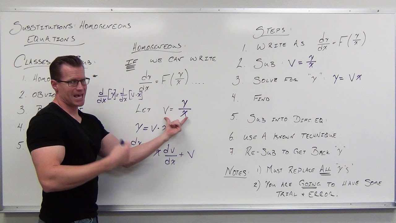
Substitutions for Homogeneous First Order Differential Equations (Differential Equations 20)
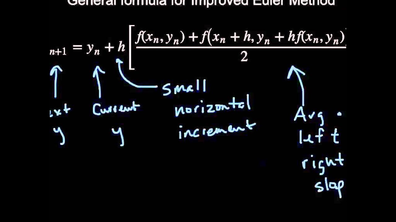
Improved Euler Method
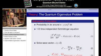
9.1 Quantum Bound Eigenstates

20.4 Heat Equation via Crank-Nickelson
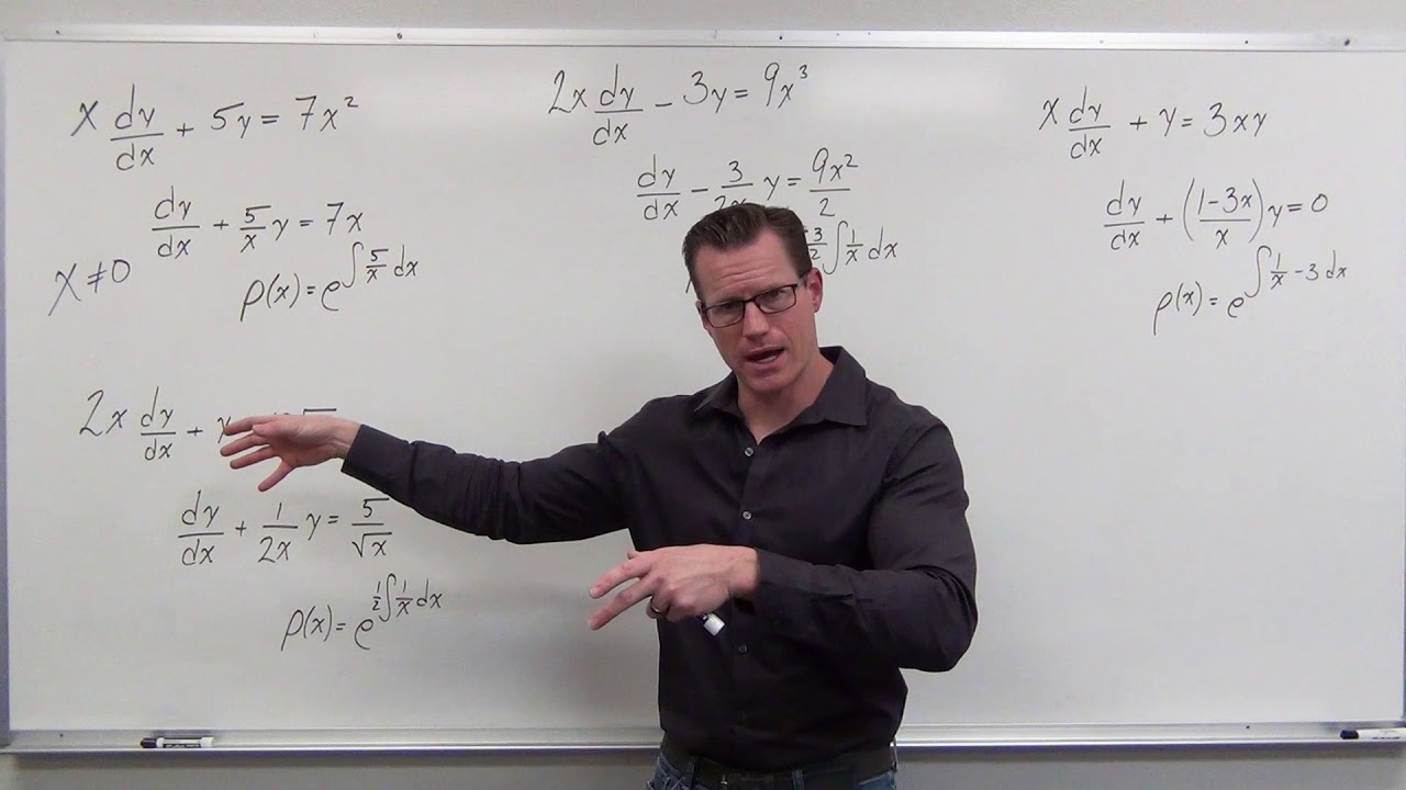
Domain Restrictions In Differential Equations and Integrating Factors (Differential Equations 17)
5.0 / 5 (0 votes)
Thanks for rating: