Calculus Chapter 5 Lecture 48 Numerical Odes II
TLDRIn this calculus lecture, Professor Greist explores the relationship between discrete and continuous mathematics, focusing on numerical methods to solve ordinary differential equations (ODEs). Starting with Euler's method, a first-order technique that approximates solutions through linearization, the lecture progresses to the more accurate midpoint and Runge-Kutta methods, which are second and fourth-order respectively. The summary emphasizes the power of these methods in approximating solutions to ODEs, illustrating the concept with examples and highlighting the importance of understanding the order of methods and their associated errors.
Takeaways
- 📚 The lecture introduces numerical methods as a way to solve ordinary differential equations (ODEs) when analytical solutions are not feasible.
- 🔍 It emphasizes the relationship between discrete and continuous calculus, highlighting how intuition from one can inform the other.
- 📉 The initial value problem for an ODE is described, focusing on approximating the final value given an initial condition and a differential equation.
- 📈 Euler's method is introduced as a simple numerical technique to approximate solutions to ODEs by using sequences and differences instead of derivatives.
- 🔢 Euler's method is explained through an update rule that projects forward the solution at each time step, based on the slope provided by the differential equation at that point.
- 📚 An example is given to illustrate Euler's method, showing how it can be used to approximate the solution to a simple exponential growth differential equation.
- 📉 The script discusses the geometric interpretation of Euler's method, describing it as a linearization that works by repeatedly approximating the solution at each time step.
- 🔍 The convergence and accuracy of Euler's method are examined, with the explanation that it is a first-order method with an error in Big O of H squared at each step.
- 📈 Two higher-order methods, the midpoint method and the Runge-Kutta method, are introduced as alternatives to Euler's method, offering better approximations at the cost of increased complexity.
- 📚 The midpoint method is described as a second-order method that uses the slope at the midpoint between time steps for a more accurate approximation.
- 🔢 The Runge-Kutta method is highlighted as a fourth-order method that provides very good approximations, with a step error in Big O of H to the fifth power and a net error in Big O of H to the fourth.
- 📉 The script concludes by comparing the different methods using a simple example, illustrating how higher-order methods can provide more accurate results.
Q & A
What is the main focus of Professor Greist's Lecture 48 on calculus?
-The main focus of the lecture is to explore the relationship between the discrete and smooth calculus, particularly how discrete calculus can help solve smooth problems, such as ordinary differential equations (ODEs).
Why might calculus fail to provide an analytical solution for some problems?
-Calculus might fail to provide an analytical solution when dealing with complex or non-separable differential equations, or when the general case cannot be solved using standard calculus methods like integration or applying an integrating factor.
What is the initial value problem for an ODE of the form dX/dt = f(x, t)?
-The initial value problem for an ODE of this form involves finding the function X(t) that satisfies the differential equation, given an initial condition X(T0) = X0, where T0 is the initial time and X0 is the initial value of X.
How does Euler's method approximate the solution to a differential equation?
-Euler's method approximates the solution by discretizing the differential equation using sequences and differences instead of derivatives. It projects forward in time using the slope at the current point to estimate the next value of X.
What is the geometric interpretation of Euler's method?
-Geometrically, Euler's method projects forward to the next time step at the current slope, which is given by the differential equation. It linearizes the problem by approximating the solution at each step.
How does the step size H affect the accuracy of Euler's method?
-The step size H affects the accuracy of Euler's method by determining the granularity of the approximation. Smaller step sizes generally lead to more accurate approximations but require more computation.
What is the difference between Euler's method and the midpoint method in terms of order?
-Euler's method is a first-order method, meaning its error is proportional to H squared. The midpoint method is a second-order method, with an error proportional to H cubed, providing a better approximation at the expense of being algebraically more complex.
What is the Runge-Kutta method and how does it compare to Euler's and midpoint methods?
-The Runge-Kutta method is a fourth-order numerical method for solving ODEs. It provides a very good approximation with a step error in O(H^5) and a net error in O(H^4), making it more accurate than both Euler's and midpoint methods, though it is also more complex.
How does the Taylor series expansion relate to Euler's method?
-Euler's method can be seen as a Taylor series expansion where all terms of order higher than one are dropped. This makes it a first-order method, as the error at each step is in O(H^2).
What is the significance of the sequence X_n in the context of Euler's method?
-In Euler's method, the sequence X_n represents the approximation of the solution at each time step. The final value X_N is an approximation of the true solution X(T) at the final time T.
Outlines
📚 Introduction to Numerical Methods in Calculus
Professor Greist introduces Lecture 48 on numerical methods in calculus, focusing on the relationship between the digital and analog worlds. The lecture aims to demonstrate how discrete calculus can be used to solve smooth calculus problems, particularly ordinary differential equations (ODEs). The professor explains that while calculus can solve some ODEs analytically, numerical methods are necessary for more complex cases. The initial value problem for an ODE is discussed, and Euler's method is introduced as a way to approximate the solution using sequences and a uniform grid. The method involves discretizing the differential equation and using the difference quotient to update the value of x at each time step.
🔍 Euler's Method: Geometric Interpretation and Examples
This paragraph delves into Euler's method, providing a geometric interpretation of how it projects forward in time using the slope information from the differential equation at the current point. The method is illustrated with a simple example involving the differential equation DX/DT = aX, where the solution is known to be exponential. The professor shows how Euler's method can approximate the solution even when the exact form is not known, as demonstrated with the example DX/DT = cos(T) + sin(X). The convergence of Euler's method with increasing number of steps is also discussed, highlighting the trade-off between accuracy and computational effort.
📈 Understanding Convergence and Error in Numerical Methods
The third paragraph explores why Euler's method works and its convergence properties by examining the Taylor series expansion of the solution around a given point. It is explained that Euler's method is a first-order method, with an error at each step proportional to the square of the time step, H. The midpoint method and the Runge-Kutta method are introduced as higher-order methods that provide better approximations at the cost of increased algebraic complexity. The Runge-Kutta method, in particular, is highlighted as a fourth-order method with an error term proportional to H to the fifth power, offering a more accurate solution for the same number of steps.
🌟 Comparing Numerical Methods and Looking Ahead
In the final paragraph, the professor compares the different numerical methods using a simple example with the differential equation DX/DT = X, where the exact solution is known to be exponential. The comparison illustrates the improvement in approximation quality as the order of the method increases, from Euler's method to the midpoint method and finally to the Runge-Kutta method. The paragraph concludes by emphasizing the importance of understanding errors in numerical methods and sets the stage for the next lecture, which will explore how discrete calculus can be used to solve problems involving definite integrals.
Mindmap
Keywords
💡Calculus
💡Numerical Methods
💡Differential Equations
💡Euler's Method
💡Discrete Calculus
💡Sequences
💡Initial Value Problem
💡Taylor Series
💡Midpoint Method
💡Runge-Kutta Method
Highlights
Introduction to numerical methods in calculus, emphasizing the relationship between discrete and smooth calculus.
Use of discrete calculus to solve smooth problems, particularly ordinary differential equations (ODEs).
Explanation of how intuition from differential calculus can inform discrete calculus and vice versa.
Overview of different classes of ODEs and methods for solving them analytically when possible.
Introduction of numerical methods as a solution when analytical methods fail for general ODEs.
Focus on the initial value problem for ODEs and the concept of approximating the final value.
Description of the process to create a uniform grid for time steps in numerical methods.
Introduction to Euler's method as a simple numerical approach to approximate solutions of ODEs.
Explanation of Euler's method from a discrete calculus perspective using sequences and differences.
Geometric interpretation of Euler's method as a linearization and projection forward in time.
Example of applying Euler's method to a simple ODE with a known analytical solution.
Demonstration of how Euler's method converges to the correct solution as the number of steps increases.
Analysis of the error in Euler's method and its relation to the Taylor series expansion.
Introduction of the midpoint method as a second-order numerical method for ODEs.
Explanation of the midpoint method's improved accuracy over Euler's method.
Introduction of the Runge-Kutta method as a higher-order numerical method.
Comparison of the accuracy and complexity of Euler's method, the midpoint method, and the Runge-Kutta method.
Conclusion emphasizing the utility of discrete methods in solving smooth calculus problems and a preview of future topics.
Transcripts
Browse More Related Video
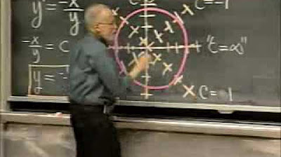
Lec 1 | MIT 18.03 Differential Equations, Spring 2006
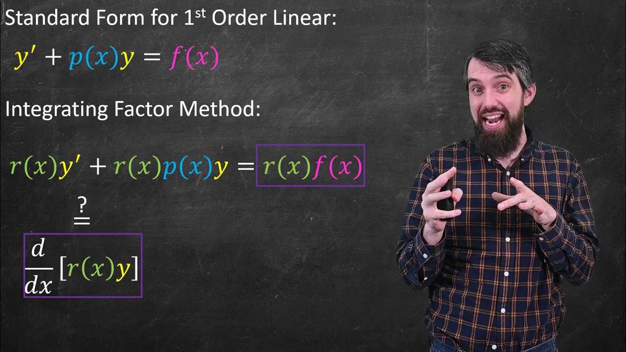
Linear Differential Equations & the Method of Integrating Factors
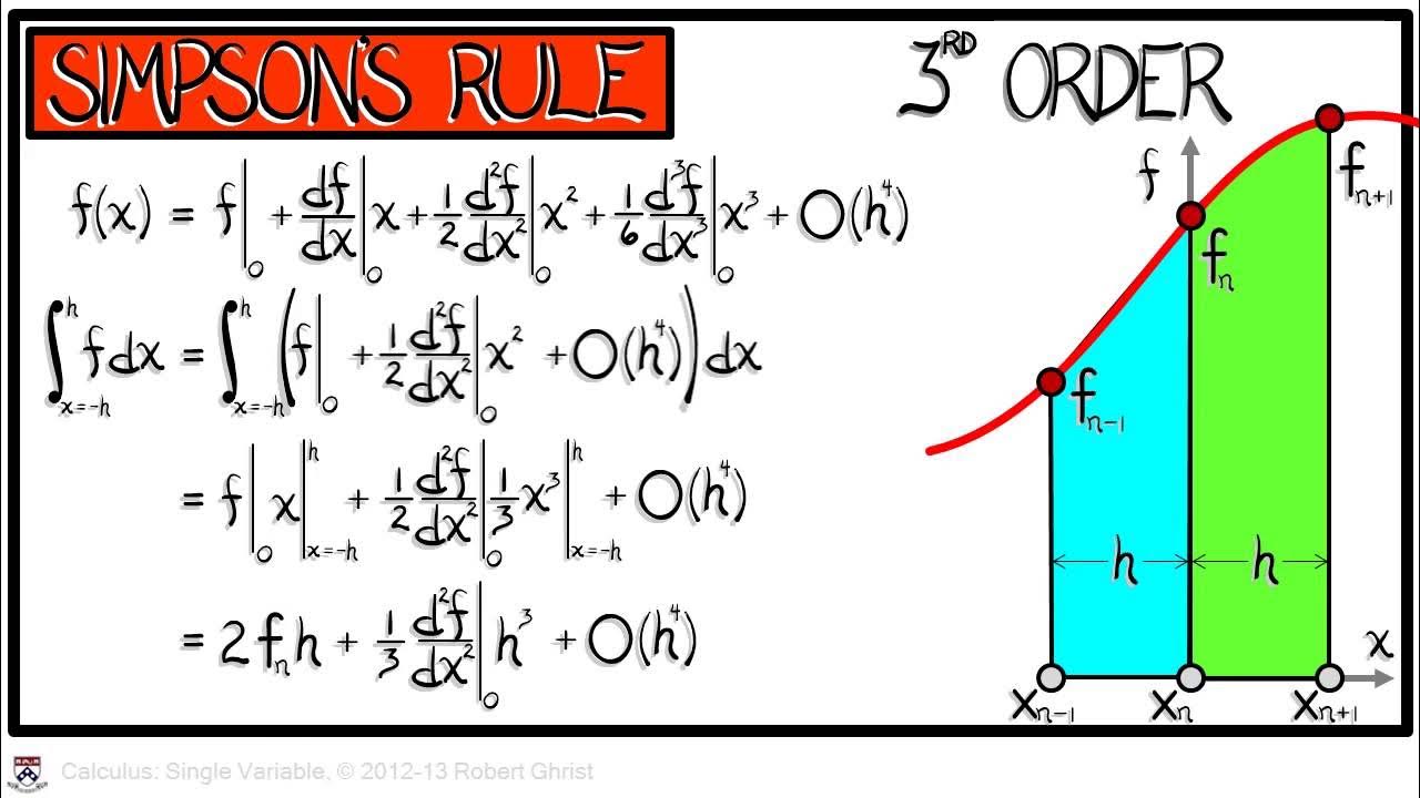
Calculus Chapter 5 Lecture 49 Numerical Integration II

8.5 ODE Algorithms
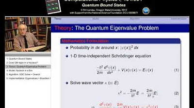
9.1 Quantum Bound Eigenstates

The Theory of 2nd Order ODEs // Existence & Uniqueness, Superposition, & Linear Independence
5.0 / 5 (0 votes)
Thanks for rating: