Derivation of Hicksian Demand Function from Utility Function

Harold Walden

20 Sept 201720:05

EducationalLearning

32 Likes 10 Comments

TLDRThis video script delves into the concept of Hicksian demand functions in economics, focusing on an optimization problem where the goal is to minimize expenditure while maintaining a fixed level of utility. The presenter uses the method of Lagrange to derive the first-order conditions, eliminating the Lagrange multiplier to find the ratio of prices to quantities. The script guides through the algebraic process of substituting these ratios back into the utility function to derive the Hicksian demand functions for two goods. It concludes with the derivation of the expenditure function, illustrating how expenditure varies with fixed utility and good prices, providing a clear example of economic optimization.

Takeaways

📚 The video discusses an economics optimization problem focusing on deriving the Hicksian demand functions for two goods.
🔍 Hicksian demand is about minimizing expenditure for a given level of utility, as opposed to Marshallian demand which maximizes utility for a given budget.
📉 The utility function provided in the script is the basis for setting up the utility minimization problem.
📝 The expenditure function is defined as the sum of the products of the prices and quantities of the two goods.
🔑 The method of Lagrange is used to incorporate the constraint of fixed utility into the minimization problem.
📈 First-order conditions are derived by differentiating the Lagrangian with respect to the quantities of goods and the Lagrange multiplier.
⚖️ The ratio of the prices of the two goods is found to be related to the quantities demanded through the first-order conditions.
🔄 Substituting the derived expressions for the quantities demanded back into the utility function helps to isolate the variables.
📐 The Hicksian demand functions for both goods are obtained by manipulating the expressions derived from the utility function.
💰 The expenditure function is derived by substituting the Hicksian demand functions into the original expenditure function.
📉 The final expenditure function shows how total expenditure varies with utility and the prices of goods, illustrating the minimized expenditure for a fixed utility level.

Q & A

What is the main focus of the video script?
-The video script focuses on explaining the concept of Hicksian demand functions in the context of an optimization problem in economics, where the goal is to minimize expenditure given a fixed level of utility.
What is the difference between a Hicksian demand function and a Marshallian demand function?
-A Hicksian demand function is concerned with minimizing expenditure to achieve a fixed level of utility, whereas a Marshallian demand function is about maximizing utility given a fixed budget or expenditure.
What is the utility function used in the script to set up the optimization problem?
-The utility function used in the script is u(x1, x2) = x1 * x2^2.
What is the expenditure function in the context of this script?
-The expenditure function is E = P1 * x1 + P2 * x2, where P1 and P2 are the prices of goods 1 and 2, respectively, and x1 and x2 are the quantities of those goods.
What method is used to solve the utility minimization problem in the script?
-The method of Lagrange multipliers is used to solve the utility minimization problem.
What are the first-order conditions derived from the Lagrangian in the script?
-The first-order conditions are the derivatives of the Lagrangian with respect to x1, x2, and the Lagrange multiplier (lambda), set equal to zero: dL/dx1 = P1 - lambda * x2^2 = 0, dL/dx2 = P2 + lambda * 2 * x1 * x2 = 0, and dL/dlambda = u - x1 * x2^2 = 0.
How are the Hicksian demand functions for x1 and x2 derived in the script?
-The Hicksian demand functions are derived by substituting the expressions for x1 and x2, which are obtained from the first-order conditions, back into the utility function and simplifying.
What is the final form of the Hicksian demand functions for x1 and x2 given in the script?
-The Hicksian demand functions are x1 = (P2^2 / (4 * P1^2))^(1/3) * U^(1/3) and x2 = 2^(1/3) * P1 / P2 * U^(1/3).
What is the expenditure function derived in the script?
-The expenditure function derived in the script is E(U, P1, P2) = (3 * U^(1/3)) / (2^(2/3) * P1^(1/3) * P2^(2/3)).
How does the script relate the concept of Hicksian demand to real-life scenarios?
-The script uses the analogy of flying from Australia to New Zealand to explain Hicksian demand, where the destination (utility level) is fixed, and the goal is to find the cheapest way (minimize expenditure) to get there.

Outlines

00:00

📚 Introduction to Hicksian Demand and Utility Minimization

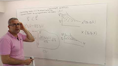
This paragraph introduces an optimization problem in economics, specifically focusing on the Hicksian demand functions for two goods. It explains the concept of minimizing expenditure to achieve a certain level of utility, contrasting it with the Marshallian approach which maximizes utility for a given budget. The script sets up the utility minimization problem, defining the expenditure function as the sum of the prices of goods multiplied by their quantities, subject to a fixed utility level determined by the consumption of goods.

05:05

🔍 Deriving Hicksian Demand Using the Lagrange Method

The paragraph explains the process of deriving an agent's Hicksian demand using the method of Lagrange. It involves setting up the Lagrangian expression with the objective function (expenditure) and the constraint (fixed utility). The first-order conditions are derived by differentiating the Lagrangian with respect to the quantities of goods, prices, and the Lagrange multiplier. These conditions are then used to eliminate the multiplier and express the ratio of prices in terms of the quantities of goods, leading to an equation that relates the quantities demanded to the utility level and prices.

10:07

📈 Calculating Optimal Demand Quantities for Hicksian Demand

This section delves into the algebraic manipulation of the first-order conditions to express the optimal demand quantities for goods in terms of utility and prices. It involves substituting the derived ratios back into the utility function and solving for the demand quantities. The process results in expressions for the Hicksian demand for both goods, which are cubic roots of utility divided by powers of price ratios, illustrating how the quantities demanded adjust with changes in utility and price levels.

15:12

💰 Deriving the Expenditure Function for Fixed Utility

The final paragraph discusses the derivation of the expenditure function when utility is held constant. It involves substituting the Hicksian demand quantities into the original expenditure function to express expenditure solely in terms of utility and prices. The resulting expenditure function is simplified to show how it varies with utility and price levels, highlighting the relationship between fixed utility, prices, and the minimized expenditure. The paragraph concludes by comparing Hicksian and Marshallian demand, emphasizing the optimization of expenditure given a fixed utility versus maximizing utility for a fixed budget.

Mindmap

Keywords

💡Economics

Economics is the social science that studies the production, distribution, and consumption of goods and services. In the video, economics is the overarching theme, as the script discusses an optimization problem within the field of economics, specifically focusing on consumer behavior and utility maximization.

💡Optimization Problem

An optimization problem in economics involves finding the best possible outcome or solution given a set of constraints. The video script describes an optimization problem where the goal is to minimize expenditure for a fixed level of utility, which is a classic economic scenario.

💡Hicksian Demand

Hicksian demand refers to the quantity of goods demanded by a consumer when the utility level is held constant, and prices are allowed to vary. The video explains how to derive Hicksian demand functions, which show the cheapest combination of goods that can provide a certain level of utility.

💡Utility Function

A utility function in economics represents the preferences of a consumer and is used to model choice behavior. In the script, the utility function is given by a mathematical expression involving the consumption of two goods, and it is the basis for the optimization problem discussed.

💡Expenditure Function

The expenditure function is the minimum amount of money a consumer needs to spend to achieve a certain level of utility, given the prices of goods. The video script involves setting up and minimizing an expenditure function as part of the Hicksian demand problem.

💡Lagrange Multiplier

In optimization problems, the Lagrange multiplier is a method used to find the local maxima and minima of a function subject to equality constraints. The script uses the method of Lagrange multipliers to derive the first-order conditions for the optimization problem.

💡First-Order Conditions

First-order conditions are a set of equations derived from the partial derivatives of a function that must be satisfied at a local extremum. In the context of the video, these conditions are used to eliminate the Lagrange multiplier and solve for the optimal quantities of goods demanded.

💡Marshallian Demand

Marshallian demand is the quantity of a good that a consumer is willing and able to purchase at a given price and income level. The video contrasts Marshallian demand with Hicksian demand, noting that the former maximizes utility for a given budget, while the latter minimizes expenditure for a given utility level.

💡Substitution

In the context of the script, substitution refers to the process of replacing one variable with another based on the relationships derived from the first-order conditions. This is a key step in solving for the Hicksian demand functions.

💡Fixed Utility

Fixed utility in the video refers to the constant level of satisfaction or preference that the consumer is trying to achieve with the least amount of expenditure. The optimization problem is set up to find the cheapest way to maintain this fixed utility level.

💡Saddle Point

A saddle point is a point on a surface where the slopes in one direction are minima and in the other direction are maxima. In the video, the script mentions looking for a saddle point when setting the first-order conditions to zero, which is part of finding the optimal solution.

Highlights

Introduction to the Hicksian demand function and its role in optimization problems in economics.

Explanation of the difference between Hicksian and Marshallian demand functions in terms of utility and budget constraints.

Setting up the utility minimization problem for deriving Hicksian demand functions.

Use of the expenditure function to represent the agent's total spending on goods.

Incorporation of the utility function as a constraint in the optimization problem.

Application of the method of Lagrange to include the constraint in the objective function.

Derivation of the first-order conditions for the optimization problem.

Elimination of the Lagrange multiplier to simplify the demand function.

Expression of the ratio of prices to quantities in the demand function.

Substitution of derived expressions back into the utility function to find Hicksian demands.

Isolation of Hicksian demand functions for goods X1 and X2 in terms of utility and prices.

Derivation of the expenditure function based on the Hicksian demands.

Explanation of how the expenditure function varies with fixed utility and prices.

Factorization of the expenditure function to simplify the expression.

Final expression of the expenditure function in terms of utility, and prices P1 and P2.

Practical analogy of Hicksian demand functions to flying from Australia to New Zealand with a fixed route.

Comparison of Hicksian and Marshallian demand functions in terms of maximizing utility for a fixed expenditure.

Encouragement for viewers to practice and enjoy economics and mathematics.

Transcripts

Browse More Related Video

How to Derive Indirect Utility and Show Homogeneous of Degree Zero

(M4E8) [Microeconomics] Consumer Surplus: Compensating and Equivalence Variations

consumer surplus and producer surplus

Optimization Problems - Calculus

Finishing the intro lagrange multiplier example

Business Calculus - Section 3.4 - Optimization and Elasticity of Demand