[H2 Chemistry] 2021 Topic 7 Chemical Equilibria 2
TLDRThis lecture delves into chemical equilibrium, focusing on the reaction quotient (Qc) and its relation to the equilibrium constant (Kc). It explains how Qc can predict the direction of equilibrium shifts and uses exercises to illustrate calculations involving Qc and Kc. The lecture also touches on Le Chatelier's principle, its limitations, and the impact of adding solvents or inert gases on equilibrium systems. It further explores the Haber process for ammonia synthesis, discussing optimal conditions and the interplay between thermodynamics and kinetics.
Takeaways
- 🧪 The lecture focuses on chemical equilibrium, specifically discussing the reaction quotient (Qc) and its role in determining the state of equilibrium in chemical reactions.
- 📚 At equilibrium, the concentrations of reactants and products remain constant, and the equilibrium constant (Kc) is used to express the balance between these species.
- 🔍 The reaction quotient (Qc) is used to predict the direction in which a reaction will proceed to reach equilibrium, based on the initial concentrations of reactants and products.
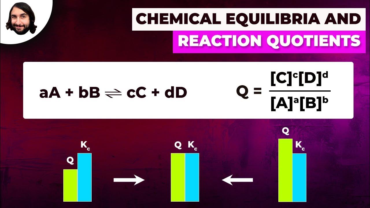
- 🤔 If Qc equals Kc, the system is already at equilibrium. If Qc is less than Kc, the reaction favors the forward direction, and if Qc is greater than Kc, the reaction favors the reverse direction.
- 📈 The lecture provides an example of the Haber process to illustrate the calculation of Qc and the determination of the direction in which the reaction will proceed to reach equilibrium.
- 💡 The concept of Le Chatelier's principle is introduced, which states that a system at equilibrium will adjust to counteract the effect of a stress, such as changes in concentration, temperature, or pressure.
- 🚫 The lecture clarifies that Le Chatelier's principle has limitations and should not be applied blindly, as it may lead to misconceptions about the behavior of equilibrium systems.
- 🌡️ The effect of adding an inert gas to an equilibrium system is discussed, highlighting that the impact on equilibrium depends on whether the system's volume is fixed or allowed to expand.
- 📉 The importance of understanding the ICE (Initial, Change, Equilibrium) table for solving equilibrium problems is emphasized, as it systematically organizes the information needed to calculate equilibrium constants and concentrations.
- 🔢 The lecture includes several exercises to practice calculating equilibrium constants and predicting the direction of reactions, reinforcing the concepts taught and the problem-solving strategies required.
- 🔄 The topic of chemical equilibrium is connected to thermodynamics, showing the relationship between Gibbs free energy (ΔG) and the equilibrium constant (K), and how ΔG can be used to predict the spontaneity and position of equilibrium.
Q & A
What is the purpose of the reaction quotient (Qc) in the context of chemical equilibrium?
-The reaction quotient (Qc) is used to determine the state of a chemical system relative to equilibrium. If Qc equals the equilibrium constant (Kc), the system is at equilibrium. If Qc is less than Kc, the reaction favors the forward direction, and if Qc is greater than Kc, the reaction favors the reverse direction.
How does the position of equilibrium shift if the reaction quotient (Qc) is less than the equilibrium constant (Kc)?
-If Qc is less than Kc, the position of equilibrium will shift to the right, favoring the forward reaction to produce more products and consume reactants until equilibrium is re-established.
What is the significance of the equilibrium constant (Kc) in expressing the concentrations of reactants and products at equilibrium?
-The equilibrium constant (Kc) is a measure of the ratio of the concentrations of products to reactants at equilibrium. It is used to predict the direction in which a reaction will proceed to reach equilibrium and to calculate the concentrations of species at equilibrium.
How does adding an inert gas at constant volume affect the equilibrium position in a gaseous reaction?
-Adding an inert gas at constant volume increases the total number of moles of gas in the system, but since the volume is fixed, the ratio of the partial pressures (or concentrations) of the reacting gases remains unchanged. Therefore, the equilibrium position does not shift.
What is the ICE table used for in chemical equilibrium problems?
-The ICE table (Initial, Change, Equilibrium) is a systematic way to organize and solve chemical equilibrium problems. It helps to keep track of the initial concentrations, the changes that occur when the system reaches equilibrium, and the final equilibrium concentrations of reactants and products.
Why is it important to consider the volume term when calculating the equilibrium constant (Kc) in terms of concentration?
-The volume term is important because it ensures that the equilibrium constant expression is based on concentrations, not just the number of moles. This is crucial for accurately predicting the direction in which the equilibrium will shift and for calculating the correct values of Kc.
How does the concept of Le Chatelier's principle apply to the addition of water to a chemical equilibrium system?
-Le Chatelier's principle states that if a stress is applied to a system at equilibrium, the system will adjust to counteract the stress. However, the principle has limitations, especially when the added substance is part of the solvent, as in the case of adding water. The concentration of the solvent remains constant, and the principle may not correctly predict the shift in equilibrium without considering the reaction quotient (Qc).
What is the significance of the equilibrium constant (Kp) in reactions involving gases?
-The equilibrium constant (Kp) is used for reactions involving gases to express the equilibrium in terms of partial pressures of the reactants and products. It is particularly useful in situations where changes in pressure or volume can affect the position of equilibrium.
How does the Haber process demonstrate the interplay between thermodynamics and kinetics?
-The Haber process, used for synthesizing ammonia, shows the interplay between thermodynamics and kinetics. Thermodynamically, lower temperatures favor the formation of ammonia, but kinetically, higher temperatures are needed to provide sufficient energy for the reaction to proceed at an industrially viable rate. A compromise temperature is chosen to balance these factors.
What is the relationship between Gibbs free energy (ΔG) and the equilibrium constant (K)?
-The relationship between Gibbs free energy (ΔG) and the equilibrium constant (K) is given by the equation ΔG = -RT ln(K), where R is the gas constant and T is the temperature in Kelvin. A negative ΔG indicates a spontaneous reaction and a position of equilibrium favoring products, while a positive ΔG indicates a non-spontaneous reaction favoring reactants.
Outlines
📘 Introduction to Reaction Quotient
The lecturer introduces the concept of the reaction quotient (Qc) in chemical equilibrium. The reaction quotient is used to calculate the concentration of reactants and products before equilibrium is reached. If Qc equals the equilibrium constant (Kc), the system is at equilibrium. If Qc is less than Kc, the reaction will proceed in the forward direction, increasing the product concentration. Conversely, if Qc is greater than Kc, the reaction will shift to the left, favoring the formation of reactants.
🔬 Application of Reaction Quotient in Haber Process
The lecturer explains how to apply the reaction quotient (Qc) using the Haber process as an example. The process involves calculating Qc for a given set of initial concentrations of nitrogen, hydrogen, and ammonia. By comparing Qc to the equilibrium constant (Kc), one can predict whether the reaction will shift to the right or left to achieve equilibrium. A detailed calculation shows that Qc is less than Kc, indicating the reaction will proceed to the right to produce more ammonia.
⚗️ Le Chatelier's Principle and Reaction Quotient
The lecturer discusses the limitations of Le Chatelier's Principle and introduces the use of Qc in specific scenarios. For example, when water is added to an aqueous solution at equilibrium, the concentration of water remains constant. Le Chatelier's Principle may not accurately predict changes, but using Qc helps to solve these issues by showing that the equilibrium will shift based on the reaction quotient's value.
🔄 Inert Gases and Equilibrium
The impact of adding inert gases to a system at equilibrium is explored. Two scenarios are considered: adding inert gas at constant pressure and constant volume. At constant pressure, the total number of moles increases, affecting Qp (reaction quotient for partial pressures) and shifting the equilibrium. At constant volume, the addition of inert gas does not affect the equilibrium position. Detailed calculations illustrate these principles.
🧪 Practical Examples of Equilibrium Shifts
Several classic equilibrium reactions, including the dimerization of NO2 and the Haber process, are used to demonstrate how changes in conditions affect the equilibrium position. For example, adding inert gas at constant pressure increases the total number of moles, affecting the reaction quotient (Qp) and shifting the equilibrium. Conversely, adding inert gas at constant volume has no effect on the equilibrium position.
📉 Calculating Equilibrium Concentrations Using ICE Tables
The lecturer demonstrates how to use ICE (Initial, Change, Equilibrium) tables to calculate equilibrium concentrations for various chemical reactions. Detailed examples, such as the dissociation of ethanoic acid in a liquid phase, show how to systematically approach these problems. By calculating the changes in concentrations and using equilibrium constants, one can determine the equilibrium concentrations of reactants and products.
🧮 Calculating Equilibrium Constants for Various Reactions
A step-by-step approach to calculating equilibrium constants for different chemical reactions is presented. Examples include the reaction of ethanoic acid with ethanol, the equilibrium between H2, I2, and HI, and the dissociation of carboxylic acids. Detailed calculations show how to set up ICE tables, calculate changes in concentration, and determine equilibrium constants (Kc) for these reactions.
🔍 Determining Equilibrium Constants from Initial Conditions
The lecturer explains how to determine equilibrium constants (Kc) from given initial conditions and equilibrium concentrations. Examples include reactions involving carboxylic acids, ethanoic acid, and esters. By using ICE tables and incorporating initial amounts and changes, the equilibrium constants for these reactions can be calculated accurately.
📊 Solving Quadratic Equations in Equilibrium Calculations
Quadratic equations often arise in equilibrium calculations, especially when determining equilibrium concentrations from initial amounts and equilibrium constants. The lecturer provides detailed examples, such as the equilibrium between H2, I2, and HI, to illustrate how to solve these quadratic equations and accurately calculate equilibrium concentrations.
🌡️ Temperature and Equilibrium Constants
The relationship between temperature and equilibrium constants (Kc and Kp) is explored. The Van't Hoff equation, which relates changes in temperature to changes in equilibrium constants, is introduced. Detailed examples show how to calculate equilibrium constants at different temperatures, considering the effects of enthalpy and entropy changes on the equilibrium position.
🔬 Practical Examples of Equilibrium Calculations
The lecturer presents more practical examples of equilibrium calculations, focusing on determining equilibrium constants (Kc and Kp) for various reactions. Examples include the dissociation of PCl5 and the reaction between H2 and I2. By using ICE tables and solving quadratic equations, the equilibrium constants for these reactions are calculated accurately.
📐 Advanced Equilibrium Calculations
Advanced equilibrium calculations are discussed, including scenarios where initial amounts and equilibrium constants are given. Examples involve reactions like the dissociation of PCl5 and the equilibrium between H2 and I2. Detailed step-by-step calculations demonstrate how to use ICE tables and solve quadratic equations to determine equilibrium concentrations and constants.
📊 Understanding Equilibrium Shifts
The lecturer explains how changes in initial conditions and equilibrium constants affect the equilibrium position. Using examples such as the reaction between H2 and I2, the impact of adding reactants or products on the equilibrium position is explored. Detailed calculations show how to predict the direction of the equilibrium shift and calculate new equilibrium concentrations.
🔄 Dynamic Equilibrium and Reaction Quotients
The concept of dynamic equilibrium and the use of reaction quotients (Qc) to predict equilibrium shifts are revisited. Examples include the decomposition of NO2 and the reaction between H2 and I2. By comparing Qc to the equilibrium constant (Kc), the direction of the equilibrium shift can be predicted accurately.
🧪 Equilibrium Calculations for Complex Reactions
Complex equilibrium calculations are discussed, including reactions involving multiple steps and components. Examples include the decomposition of NO2 and the equilibrium between CO, H2, and methanol. Detailed step-by-step calculations show how to determine equilibrium constants and predict equilibrium positions for these complex reactions.
📊 Practical Application of Equilibrium Concepts
The practical application of equilibrium concepts in industrial processes, such as the Haber process for ammonia synthesis, is discussed. The interplay between thermodynamics and kinetics in optimizing reaction conditions is explored. Detailed examples show how to balance temperature, pressure, and catalyst use to maximize product yield while maintaining economic feasibility.
🔬 Experimental Determination of Equilibrium Constants
Methods for experimentally determining equilibrium constants (Kc and Kp) are presented. Examples include titration of equilibrium mixtures and using colorimetry for complex ion equilibria. The importance of maintaining constant temperature and accurately measuring concentrations is emphasized. Practical tips for designing experiments to determine equilibrium constants are provided.
📉 Linking Equilibrium Constants and Gibbs Free Energy
The relationship between equilibrium constants (K) and Gibbs free energy (ΔG) is explored. The lecturer explains how ΔG determines the direction of the reaction and the position of equilibrium. The mathematical relationship between ΔG and K, including the use of the Van't Hoff equation, is discussed. Examples show how changes in temperature affect ΔG and K, influencing the equilibrium position.
📘 Summary and Advanced Topics in Equilibrium
The lecturer provides a summary of key concepts in chemical equilibrium, including the use of reaction quotients (Qc), equilibrium constants (Kc and Kp), and the relationship between ΔG and K. Advanced topics, such as the Van't Hoff equation and the impact of temperature on equilibrium constants, are revisited. The importance of understanding these concepts for future studies in chemistry, including acid-base and solubility equilibria, is emphasized.
🔬 Practical Tips for Equilibrium Calculations
Practical tips for performing accurate equilibrium calculations are provided. The lecturer emphasizes the importance of using ICE tables, carefully tracking changes in concentrations, and accurately solving quadratic equations. Examples from previous sections are revisited to reinforce key points and demonstrate best practices for equilibrium calculations.
Mindmap
Keywords
💡Chemical Equilibrium
💡Equilibrium Constant (Kc or Kp)
💡Reaction Quotient (Qc or Qp)
💡Le Châtelier's Principle
💡Haber Process
💡ICE Table
💡Stoichiometry
💡Gibbs Free Energy (ΔG)
💡Catalyst
💡Exothermic Reaction
Highlights
Introduction to the concept of the reaction quotient (Qc) and its distinction from the equilibrium constant (Kc).
Explanation of how to calculate Qc using initial concentrations of reactants and products.
Discussion on the significance of comparing Qc to Kc to determine the direction of the reaction.
Illustration of how a reaction will shift to the right if Qc < Kc and to the left if Qc > Kc.
Example calculation of Qc for the Haber process and its application in predicting the direction of the reaction shift.
Explanation of the use of ICE tables (Initial, Change, Equilibrium) for systematic problem-solving in chemical equilibrium.
Introduction to Le Chatelier’s Principle and its limitations in predicting the effect of changes in conditions on equilibrium.
Explanation of how adding an inert gas at constant volume does not affect the position of equilibrium.
Demonstration of how equilibrium shifts with changes in concentration, pressure, and temperature using specific examples.
Detailed example of calculating equilibrium concentrations for a reaction involving ethanoic acid and ethanol.
Introduction to the concept of Gibbs free energy (ΔG) and its relationship with the equilibrium constant (K).
Explanation of the significance of ΔG being negative, zero, or positive and its impact on the position of equilibrium.
Discussion on the derivation of the Van’t Hoff equation and its use in predicting how equilibrium constants change with temperature.
Example calculation of equilibrium constants for various reactions using provided data.
Application of the concepts in a real-world context, specifically the Haber process for ammonia synthesis.
Explanation of the optimal conditions for the Haber process, balancing kinetics and thermodynamics for maximum efficiency.
Overview of the practical considerations and economic factors in industrial chemical processes.
Introduction to the use of catalysts to accelerate reactions and achieve equilibrium more quickly.
Transcripts
Browse More Related Video

18. Introduction to Chemical Equilibrium

Le Chatelier's principle | Chemical equilibrium | Chemistry | Khan Academy

Chemical Equilibrium Full Topic Video

ALEKS: Using an equilibrium constant to predict the direction of a spontaneous reaction

Le Chatelier's principle: Worked example | Chemical equilibrium | Chemistry | Khan Academy
Chemical Equilibria and Reaction Quotients
5.0 / 5 (0 votes)
Thanks for rating: