Sampling Distributions: Introduction to the Concept
TLDRThis script introduces the fundamental concept of sampling distributions in statistics, which are crucial for statistical inference. It explains that the sampling distribution of a statistic is its probability distribution, obtained by repeatedly drawing samples from a population. The script uses an example of a university class to illustrate how a professor, without access to the exact average age of students, can estimate it using a sample mean. It further explains that the sample mean varies with each sample drawn and demonstrates through a computer simulation how a histogram of many sample means closely resembles the true sampling distribution. The concept is essential for making statistical inferences about population parameters, such as expressing confidence intervals.
Takeaways
- 📚 The concept of sampling distributions is foundational to statistical inference techniques.
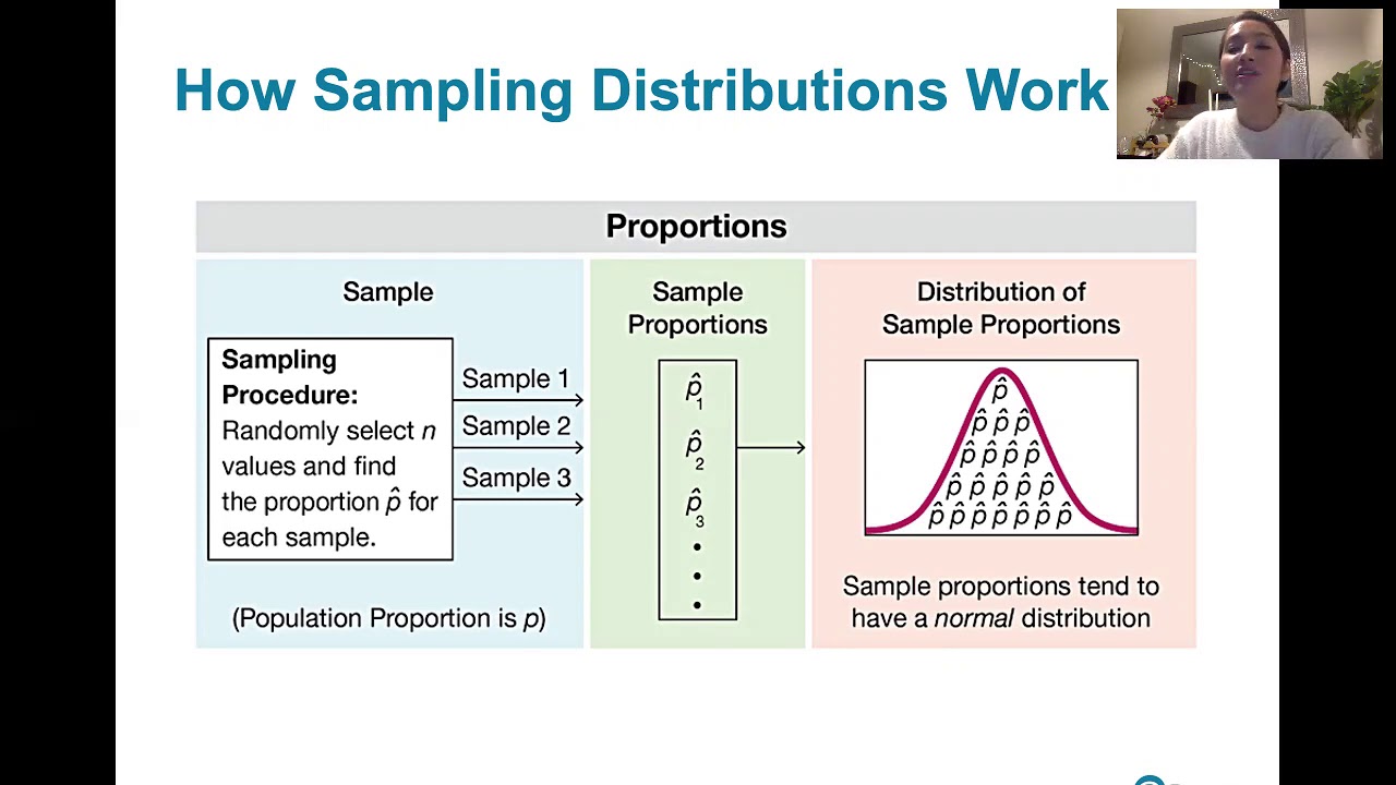
- 🔍 A sampling distribution is the probability distribution of a statistic, showing how it varies with repeated sampling from the population.
- 👨🏫 The example of a university class with 16 students illustrates the concept, where the average age is a parameter of interest.
- 🔢 The true population mean (mu) is an unknown value that the professor wishes to estimate.
- 🎯 The professor can take a sample of three students to estimate the population mean, representing a practical approach to statistical inference.
- 📉 The true ages of the students and the calculated true population mean are not known to the professor, emphasizing the role of estimation.
- 📈 The sample mean is used as an estimator for the unknown population mean, providing a point estimate.
- 🤔 The uncertainty associated with the sample mean is a key concern, which is addressed by examining the sampling distribution.
- 📊 Repeated sampling leads to different sample means, highlighting the variability inherent in statistical estimation.
- 📚 The histogram of sample means, if plotted from many repeated samples, would resemble the true sampling distribution of the sample mean.
- 🧐 The sampling distribution is crucial for making inferences about population parameters, such as expressing confidence intervals.
Q & A
What is the main concept discussed in the script?
-The main concept discussed in the script is the sampling distribution of a statistic, which is the probability distribution of that statistic if samples were to be repeatedly drawn from the population.
Why is understanding the sampling distribution important for statistical inference?
-Understanding the sampling distribution is crucial for statistical inference because it allows us to make statements about population parameters based on mathematical arguments related to the sampling distribution of a statistic.
What is the difference between a parameter and a statistic?
-A parameter is a numerical characteristic of a population, such as the population mean (mu), while a statistic is a numerical characteristic of a sample, such as the sample mean (X bar), used to estimate the parameter.
How does the script illustrate the concept of sampling distribution with an example?
-The script uses the example of a university class with 16 students where the professor wants to know the average age of the students. It explains how the sample mean (X bar) varies with different samples drawn from this population.
What is the true population mean (mu) in the example provided?
-The true population mean (mu) in the example is 239.8125, which is calculated by taking the average of the ages of the 16 students.
Why is the professor unable to know the true population mean (mu) in the example?
-In the example, it is assumed that the professor does not have access to the records that contain the true ages of the students, making mu an unknown quantity to the professor.
How does the script demonstrate the variability of the sample mean?
-The script demonstrates the variability of the sample mean by drawing different samples of three students from the class and calculating the sample mean for each, showing how it varies from one sample to another.
What does the script imply about the shape of the sampling distribution of the sample mean?
-The script implies that in many situations, the sampling distribution of the sample mean is approximately normal, although it does not look like that in the specific example provided.
What is the significance of the histogram of sample means shown in the script?
-The histogram of sample means is significant because it represents the distribution of the sample means obtained from repeated sampling, closely resembling the true sampling distribution of the sample mean in that scenario.
How does the script relate the concept of sampling distribution to uncertainty and confidence intervals?
-The script relates the concept of sampling distribution to uncertainty and confidence intervals by explaining that we can use the sampling distribution to make statements about how close our sample mean estimate is likely to be to the true population mean (mu), and to construct confidence intervals.
What is the practical implication of the sampling distribution in real-world scenarios?
-In real-world scenarios, the concept of a sampling distribution is important because it helps us understand that the value of a statistic we observe in our sample is a random draw from that statistic's sampling distribution, which is crucial for making inferences about the population.
Outlines
📚 Introduction to Sampling Distributions
This paragraph introduces the fundamental concept of sampling distributions, which are the basis for statistical inference techniques. It explains that the sampling distribution of a statistic is its probability distribution when samples are repeatedly drawn from a population. The paragraph uses an example of a university class with 16 students to illustrate how the average age (a parameter denoted as mu) can be estimated through sampling. It also discusses the variability of the sample mean and how it can be used to estimate the unknown population mean. The concept of uncertainty associated with the sample mean is introduced, and the paragraph concludes with a mention of using mathematical arguments based on the sampling distribution to understand how close the sample mean is likely to be to the true value of mu.
📊 Understanding the Sample Mean's Distribution
This paragraph delves deeper into the concept of the sample mean's distribution, emphasizing its importance in statistical inference. It uses the same university class example to demonstrate how the sample mean can vary with different samples and how this variation can be visualized through a histogram. The paragraph explains that in many cases, the sample mean's distribution is approximately normal, and it discusses the idea of calculating the exact sampling distribution in a scenario where the sample size is small relative to the population size. The paragraph also highlights that while in practice we typically draw only one sample, the concept of the sampling distribution is crucial for making statements about population parameters. It concludes by noting that confidence intervals, such as being 95% confident that the sample mean lies within 22.1 units of mu, are derived from mathematical arguments related to the sampling distribution of the sample mean.
Mindmap
Keywords
💡Sampling Distribution
💡Statistical Inference
💡Parameter
💡Sample Mean (X bar)
💡Population Mean (mu)
💡Random Sample
💡Uncertainty
💡Histogram
💡Normal Distribution
💡Confidence Interval
Highlights
The concept of sampling distributions is fundamental to statistical inference techniques.
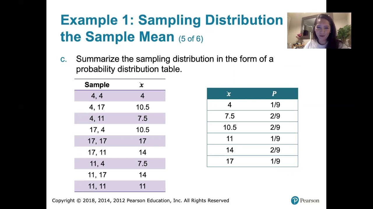
The sampling distribution of a statistic is its probability distribution when samples are repeatedly drawn from the population.
A statistic's sampling distribution shows how the statistic varies from sample to sample.
An example of a university class with 16 students is used to illustrate the concept of sampling distribution.
The average age of the students represents the population parameter, denoted as mu.
The professor, as an example, does not have access to the true average age (mu) and must estimate it.
The professor can take a sample of three students to estimate the average age.
The true ages of the students and the calculated true population mean (mu = 239.8125) are unknown to the professor.
A random sample of three students is selected, and their ages are used to calculate a sample mean.
The sample mean is used to estimate the unknown population mean (mu).
The concept of uncertainty is introduced, questioning how close the sample mean is likely to be to the true mu.
The sampling distribution of the sample mean (X bar) is used to understand the uncertainty.
Repeated sampling illustrates that the sample mean will vary, and this variation is depicted through a histogram.
The histogram of sample means closely resembles the true sampling distribution when many samples are taken.
The population mean (mu) is often approximated by the distribution of the sample mean, which is often normally distributed.
The number of possible samples (16 choose 3) gives another perspective on the sampling distribution.
In practice, only one sample is typically drawn, but the concept of the sampling distribution is crucial for statistical inference.
Mathematical arguments based on the sampling distribution allow making statements about population parameters with confidence intervals.
Transcripts
Browse More Related Video
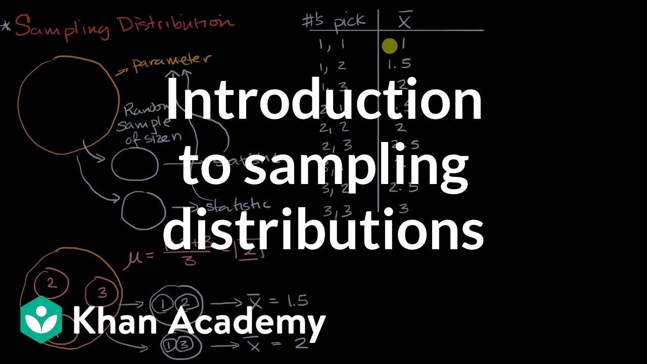
Introduction to sampling distributions | Sampling distributions | AP Statistics | Khan Academy
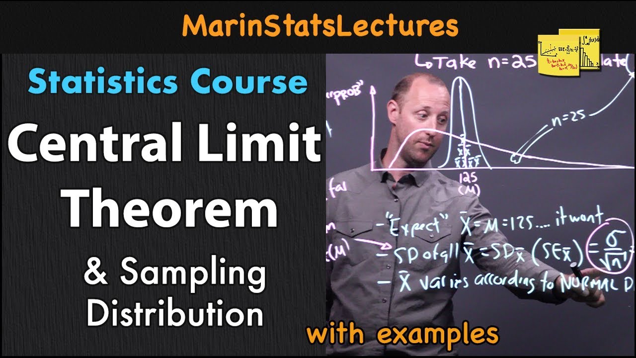
Central Limit Theorem & Sampling Distribution Concepts | Statistics Tutorial | MarinStatsLectures
6.3.1 Sampling Distributions and Estimators - Sampling Distributions Described and Defined
6.3.3 Sampling Distributions and Estimators - Sampling Distribution of the Sample Means
Confidence Interval Concept Explained | Statistics Tutorial #7 | MarinStatsLectures
SAMPLING DISTRIBUTION OF SAMPLE MEANS - WITH AND WITHOUT REPLACEMENT
5.0 / 5 (0 votes)
Thanks for rating: