BusCalc 06 Rates of Change
TLDRThe video script delves into the concept of rates of change, focusing on two types: average and instantaneous rates of change. The presenter uses the analogy of a road trip to explain average speed, which is the total distance driven divided by the time taken. Instantaneous speed, on the other hand, is the speed at a specific moment and is derived using limits in calculus. The script further illustrates these concepts with examples, including a detailed calculation of the instantaneous rate of change of a quadratic function. It concludes with an application of these concepts to calculate the average rate of change in the stock price of ExxonMobil from January 1, 2018, to the present, demonstrating how calculus can be applied to real-world scenarios.
Takeaways
- 📚 The video discusses rates of change, focusing on two types: average rates of change and instantaneous rates of change.
- 🚗 The average speed is calculated by dividing the total distance traveled by the total time taken, which is a measure of the average rate of change of distance over time.
- 📈 The instantaneous rate of change, unlike the average, focuses on the rate of change at a specific point, which can be found by taking a limit as the time interval approaches zero.
- 🛣️ An example given is a road trip from Midland to Santa Fe, New Mexico, to illustrate the concept of average speed over a distance of 400 miles in 8 hours.
- ⏱️ The video explains that actual driving speed varies throughout a trip, with moments of speeding up and slowing down, which is not captured by the average speed alone.
- 📊 The concept of a distance-time graph is introduced to visualize the trip, with the steepness of the graph representing the speed at different times during the journey.
- 🚦 Another example involves driving from a driveway to a stop sign, with the graph's slope changing to reflect acceleration and deceleration.
- 🔢 The instantaneous speed is the speed at a specific moment, which can be approximated by calculating the average speed over an extremely small time interval.
- 🧮 Mathematically, the instantaneous rate of change is found using the limit as the change in the independent variable approaches zero, which is a fundamental concept in calculus.
- 📉 The average rate of change is calculated by taking the difference in function values over the difference in the input values, which is applicable to various real-world scenarios, such as stock price changes over time.
- 💡 The video concludes by demonstrating how to calculate the average rate of change for the stock price of ExxonMobil from January 1, 2018, to January 22, 2022, using data obtained from a Google search and Microsoft Excel.
Q & A
What are the two types of rates of change discussed in the video?
-The two types of rates of change discussed are average rates of change and instantaneous rates of change.
What is the formula for calculating the average speed of a trip?
-The average speed is calculated by dividing the total distance traveled by the total time taken for the trip.
How does the speedometer in a car measure speed?
-The speedometer measures speed in miles per hour (mph), which is a ratio of miles traveled to the time taken to travel that distance.
What does the graph of distance versus time represent?
-The graph of distance versus time represents the rate of change of distance over time, showing how the distance traveled changes with the passage of time.
How does the steepness of the graph in a distance-time plot relate to speed?
-The steepness of the graph in a distance-time plot is directly related to speed. A steeper graph indicates a higher rate of change, which means a faster speed.
What is the instantaneous rate of change?
-The instantaneous rate of change is the rate of change at a specific point, calculated using the limit as the time interval approaches zero.
How can you estimate the instantaneous speed at a particular time by using the average speed?
-You can estimate the instantaneous speed at a particular time by calculating the average speed over an extremely small time interval close to that time.
What is the formula for the average rate of change of a function over an interval?
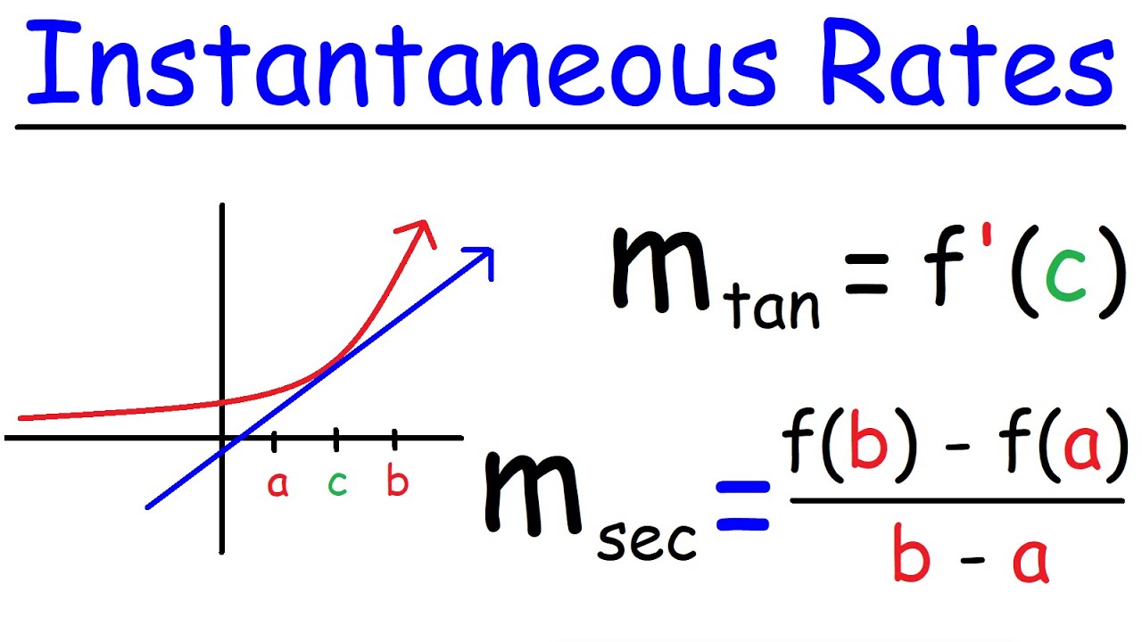
-The formula for the average rate of change is (f(b) - f(a)) / (b - a), where 'a' is the start point and 'b' is the end point of the interval.
How is the instantaneous rate of change related to the concept of limits in calculus?
-The instantaneous rate of change is calculated using the concept of limits, specifically taking the limit as the change in the independent variable (h) approaches zero.
What is the instantaneous rate of change of the function f(x) = x^2 at the point x = 5?
-The instantaneous rate of change of the function f(x) = x^2 at the point x = 5 is 10, as calculated using the formula for instantaneous rate of change and substituting x with 5.
How can you calculate the average rate of change of a stock price over a period of time?
-You can calculate the average rate of change of a stock price over a period of time by finding the difference in the stock price between the start and end dates, and dividing it by the number of time units (days, years, etc.) that have passed.
Outlines
🚗 Understanding Average and Instantaneous Rates of Change
This paragraph introduces the topic of rates of change, specifically focusing on average and instantaneous rates. It uses the example of a road trip from Midland to Santa Fe, New Mexico, to explain average speed as a ratio of distance to time. The speaker emphasizes that while the average speed might be 50 miles per hour, there would be times during the trip where the speed would vary, either faster or slower. The concept of a speedometer reading (mph) is also discussed to illustrate the idea of speed as a rate of change.
📈 Graphing Distance vs. Time with Stops and Speed Variations
The speaker continues the discussion by graphing the distance traveled over time, including the concept of stops during a trip which are represented as horizontal lines on the graph since no distance is covered during these time intervals. The paragraph explores how the graph's steepness can indicate faster speeds and how the graph would appear if the speed varied, with steeper sections representing faster driving and shallower sections indicating slower speeds. The concept of speed as the rate of change of distance over time is highlighted.
🚦 Analyzing Speed Changes Over Short Time Intervals
The paragraph delves into the specifics of calculating average speed over short time intervals using the example of driving from a driveway to a stop sign. It discusses how speed changes when starting from a stop, accelerating, and then decelerating to a stop again. The speaker uses a table of values to calculate average speeds over different time intervals and introduces the concept of instantaneous speed at a specific time, which is the speed at a precise moment rather than an average over an interval.
📉 Calculating Average Speed Over Different Time Intervals
This section focuses on calculating the average speed for different time intervals during a trip. It provides a detailed method for finding the average speed between two points in time using the distance traveled and the time elapsed. The speaker also touches on the idea of instantaneous speed, which is the speed at a specific moment in time, and differentiates it from average speed, which is calculated over a period of time.
🔍 Instantaneous Speed and the Concept of Limits
The paragraph explains the mathematical concept of instantaneous speed and how it is derived from the average speed by taking an infinitely small time interval. It introduces the formal mathematical definitions of average rate of change and instantaneous rate of change, with the latter involving a limit as the time interval approaches zero. The speaker illustrates how to calculate the instantaneous rate of change at a specific point using the concept of limits.
🧮 Applying the Instantaneous Rate of Change Formula
The speaker provides an example of using the instantaneous rate of change formula with a function f(x) = x^2 at the point x = 5. It walks through the algebraic process of applying the formula, factoring out common terms, and simplifying to find the instantaneous rate of change. The example demonstrates how the formula can be used to determine the rate of change at any given point in the function.
📉 Calculating the Average Rate of Change of a Stock Price
The final paragraph applies the concept of average rate of change to real-world data, specifically the stock price of ExxonMobil from January 1, 2018, to the present day. The speaker outlines the steps to calculate the average rate of change using the stock price at two different dates and the time elapsed between them. It concludes with a calculation of the average rate of change in dollars per year, illustrating how the stock price has been decreasing on average over the specified period.
📊 Understanding the Difference Between Average and Instantaneous Rates of Change
This paragraph summarizes the key differences between average and instantaneous rates of change. It emphasizes that while average rate of change considers the overall trend over a period, instantaneous rate of change focuses on the specific rate at a precise moment. The speaker also notes that the concepts discussed are applicable to various fields and are useful for understanding and modeling real-world phenomena.
Mindmap
Keywords
💡Rates of Change
💡Average Speed
💡Instantaneous Speed
💡Limit
💡Distance Function
💡Stock Price
💡Excel
💡Graph
💡Speedometer
💡Algebra
💡Function
Highlights
The video discusses rates of change, focusing on average and instantaneous rates of change.
Average rate of change is introduced as the ratio of distance traveled to time taken, measured in miles per hour (mph).
Instantaneous rate of change is explained as the rate of change at a specific point in time, as opposed to an average over a period.
An example of a road trip from Midland to Santa Fe, New Mexico, is used to illustrate the calculation of average speed.
The concept of speedometers and how they measure speed in mph is explained.
The video uses a graph to visualize the trip, showing stops and the overall distance-time relationship.
The difference between driving at a constant speed and varying speeds throughout a trip is discussed.
The video demonstrates how to calculate the average speed for different segments of a trip using a table of values.
Instantaneous speed is explored through the concept of taking an infinitely small time interval around a specific time point.
The mathematical formula for average rate of change is derived and explained.
The concept of a limit is introduced in the context of calculating instantaneous rate of change.
An example calculation is performed to find the instantaneous rate of change of a quadratic function at a specific point.
The video concludes with a real-world application, calculating the average rate of change of ExxonMobil's stock price over a period of time.
Google and Microsoft Excel are utilized to find current stock prices and perform calculations for the average rate of change.
The impact of using different units (e.g., dollars per day vs. dollars per year) on the interpretation of the average rate of change is discussed.
The video emphasizes the difference between average and instantaneous rates of change and their respective calculations.
The practical significance of rates of change in various fields such as economics, business, and engineering is highlighted.
The use of limits from calculus to determine rates of change in real-world scenarios is demonstrated.
Transcripts
5.0 / 5 (0 votes)
Thanks for rating:


