Probability is not Likelihood. Find out why!!!
TLDRIn this engaging StatQuest video, host Josh Dahmer explains the nuanced difference between probability and likelihood, two concepts that are often confused. Using a normal distribution as an example, he illustrates how probability is calculated as the area under the curve between two points, such as the chance of a mouse weighing between 32 and 34 grams, which is 29%. In contrast, likelihood is a measure of how well a particular distribution fits a fixed data point; for instance, the likelihood of a 34-gram mouse given a distribution with a mean of 32 grams and a standard deviation of 2.5 is 0.12. The video clarifies that probabilities are about fixed distributions with variable data, while likelihoods consider fixed data with variable distribution parameters. Dahmer encourages viewers to explore further by checking out the maximum likelihood estimator derivation for the exponential distribution on StatQuest.
Takeaways
- 📊 **Understanding Probability vs. Likelihood**: The video explains the difference between probability and likelihood, two concepts that are often confused.
- 🐭 **Normal Distribution Example**: The example of mouse weights with a normal distribution is used to illustrate the concepts, which applies to all continuous distributions.
- 🔢 **Probability Calculation**: Probability is represented as the area under the curve of a distribution, in this case, the chance of a mouse weighing between 32 and 34 grams is 29%.
- 📈 **Notation of Probability**: Mathematically, probability is expressed as P(Data | Parameters), where the parameters define the distribution and the data is fixed.
- ⚖️ **Changing Probability**: By altering the left side of the probability equation, one can calculate the probability for different scenarios, such as a mouse weighing more than 34 grams.
- 📋 **Fixed Measurements in Likelihood**: Unlike probability, likelihood involves fixed data points and allows for the distribution to be shifted or modified.
- 📉 **Likelihood Calculation**: The likelihood of a 34-gram mouse is a specific point on the curve with a value of 0.12, which changes if the distribution's mean is altered.
- 🔧 **Adjusting the Distribution**: The shape and location of the distribution can be modified by changing the mean, which affects the likelihood of observing certain data points.
- 📐 **Mathematical Representation of Likelihood**: Likelihood is written as L(Parameters | Data), indicating that the distribution parameters are variable given fixed data.
- 📚 **Further Learning**: The video encourages viewers to check out other StatQuest videos for more detailed mathematical derivations, such as the maximum likelihood estimator for the exponential distribution.
- 🎶 **Supporting StatQuest**: The presenter, Josh Dahmer, invites viewers to subscribe for more content and to support the channel by purchasing his original songs on Bandcamp.
Q & A
What is the main topic discussed in the video script?
-The main topic discussed in the video script is the difference between probability and likelihood in the context of statistical distributions.
What are the two closely related concepts that are often confused?
-The two closely related concepts that are often confused are probability and likelihood.
What is an example of a continuous distribution used in the script?
-An example of a continuous distribution used in the script is the normal distribution of mouse weights.
What is the mean and standard deviation of the mouse weight distribution in the example?
-In the example, the mean of the mouse weight distribution is 32 grams and the standard deviation is 2.5 grams.
What does the area under the curve in a probability distribution represent?
-The area under the curve in a probability distribution represents the probability or the likelihood of a certain event occurring, such as the weight of a randomly selected mouse falling within a specific range.
What is the probability that a randomly selected mouse weighs between 32 and 34 grams?
-The probability that a randomly selected mouse weighs between 32 and 34 grams is 29%, which is represented by the area under the curve between these two values.
How is the likelihood of a distribution with a specific mean and standard deviation given a weighed mouse calculated?
-The likelihood is calculated as the y-axis value at the point corresponding to the fixed data point (in this case, the weight of the mouse) on the distribution curve.
What happens if you shift the mean of the distribution to match the weight of the mouse in the likelihood calculation?
-If you shift the mean of the distribution to match the weight of the mouse, the new likelihood value would change, reflecting the new position of the distribution relative to the data point.
What is the mathematical notation used to express the likelihood of a distribution given a weighed mouse?
-The mathematical notation for the likelihood is written as the likelihood of a distribution with a specific mean and standard deviation, given the weight of the mouse, which equals a specific value (in the script, 0.12).
How are probabilities and likelihoods different in terms of their mathematical representation?
-Probabilities are represented as the area under a fixed distribution curve given certain parameters (like mean and standard deviation), while likelihoods are represented as the y-axis values for fixed data points with distributions that can be moved or adjusted.
What does the video script suggest for further understanding of the equations related to likelihoods?
-The video script suggests checking out the StatQuest episode that derives the maximum likelihood estimator for the exponential distribution for further understanding of the equations related to likelihoods.
How can viewers support StatQuest and get more content?
-Viewers can support StatQuest by subscribing to the channel and considering the purchase of original songs by the host, Josh Dahmer, which can be found on his Bandcamp page linked in the video description.
Outlines
📊 Understanding Probability and Likelihood
In this paragraph, Josh Dahmer introduces the topic of the video: the difference between probability and likelihood. He emphasizes the importance of visualizing these concepts, particularly through the lens of a normal distribution. The video uses the example of a distribution of mouse weights with a mean of 32 grams and a standard deviation of 2.5 grams to illustrate the concept of probability. The probability of selecting a mouse weighing between 32 and 34 grams is calculated as the area under the curve, which is 29%. This is represented mathematically as P(data | distribution), where 'data' refers to the mouse's weight and 'distribution' refers to the parameters of the normal distribution. The video also touches on how to calculate different probabilities by changing the 'data' part of the equation while keeping the 'distribution' parameters constant.
🐭 Fixed Data and Variable Distributions in Likelihood
This paragraph delves into the concept of likelihood, which is approached from the perspective of having already obtained data (in this case, the weight of a mouse). The likelihood of weighing a 34-gram mouse is represented by a point on the curve with a value of 0.12, and is mathematically expressed as L(distribution | data). Unlike probability, where the distribution is fixed and the data is variable, in likelihood, the data point is fixed, and the distribution can be shifted or varied. The video demonstrates this by showing how the likelihood changes if the mean of the distribution were to shift to 34 grams, resulting in a new likelihood value of 0.21. This section clarifies the fundamental difference between probability, which is about the area under a curve given a distribution, and likelihood, which is about the height of the curve at a fixed data point with a variable distribution.
🔢 Mathematical Expression of Probability and Likelihood
The video concludes with a summary of the key differences between probability and likelihood. Probability is defined as the area under a fixed distribution curve corresponding to the data, mathematically expressed as P(data | distribution). On the other hand, likelihood is the value on the y-axis of the distribution curve for a given fixed data point, which can vary the distribution, expressed as L(distribution | data). The video encourages viewers to check out another StatQuest episode for the derivation of the maximum likelihood estimator for the exponential distribution. Josh also invites viewers to subscribe for more content and to support the channel by purchasing his original songs, with a link provided in the comments section.
Mindmap
Keywords
💡Probability
💡Likelihood
💡Normal Distribution
💡Mean
💡Standard Deviation
💡Continuous Distribution
💡Area Under the Curve
💡Data Given a Distribution
💡Distribution Given Data
💡Maximum Likelihood Estimator
💡StatQuest
Highlights
The video explains the difference between probability and likelihood, two concepts that are often confused.
Probability is demonstrated using a normal distribution, specifically a distribution of mouse weights with a mean of 32 grams and a standard deviation of 2.5 grams.
The area under the curve between 32 and 34 grams represents a 29% chance of a randomly selected mouse weighing within that range.
Probability is mathematically notated as the likelihood of weighing a mouse between certain weights given the mean and standard deviation of the distribution.
The concept of probability applies to all continuous distributions, not just the normal distribution.
Likelihood is introduced as a concept that assumes you have already measured a specific data point, such as the weight of a mouse.
The likelihood of weighing a 34 gram mouse is a specific point on the curve with a value of 0.12.
Likelihood is mathematically expressed as the distribution given a fixed data point, with the ability to modify the distribution's shape and location.
If the mean of the distribution is shifted, the likelihood value changes, illustrating the dependency of likelihood on the distribution's parameters.
In summary, probabilities are areas under a fixed distribution, while likelihoods are y-axis values for fixed data points with adjustable distributions.
The video provides a clear distinction between the two concepts, emphasizing their different applications in statistical analysis.
The presenter, Josh Dahmer, occasionally mixes up the concepts himself, showing the complexity and common confusion between them.
The video uses visual aids to clarify the abstract statistical concepts, making them more accessible to viewers.
The presenter encourages viewers to check out another StatQuest video that derives the maximum likelihood estimator for the exponential distribution.
The video concludes with a call to action for viewers to subscribe for more content and support the channel by purchasing original songs.
The presenter's original songs are available for purchase on Bandcamp, with a link provided in the video description.
The video is part of the StatQuest series, which aims to make statistical concepts more understandable through engaging explanations.
Transcripts
Browse More Related Video

Data Science & Statistics Tutorial: The Poisson Distribution
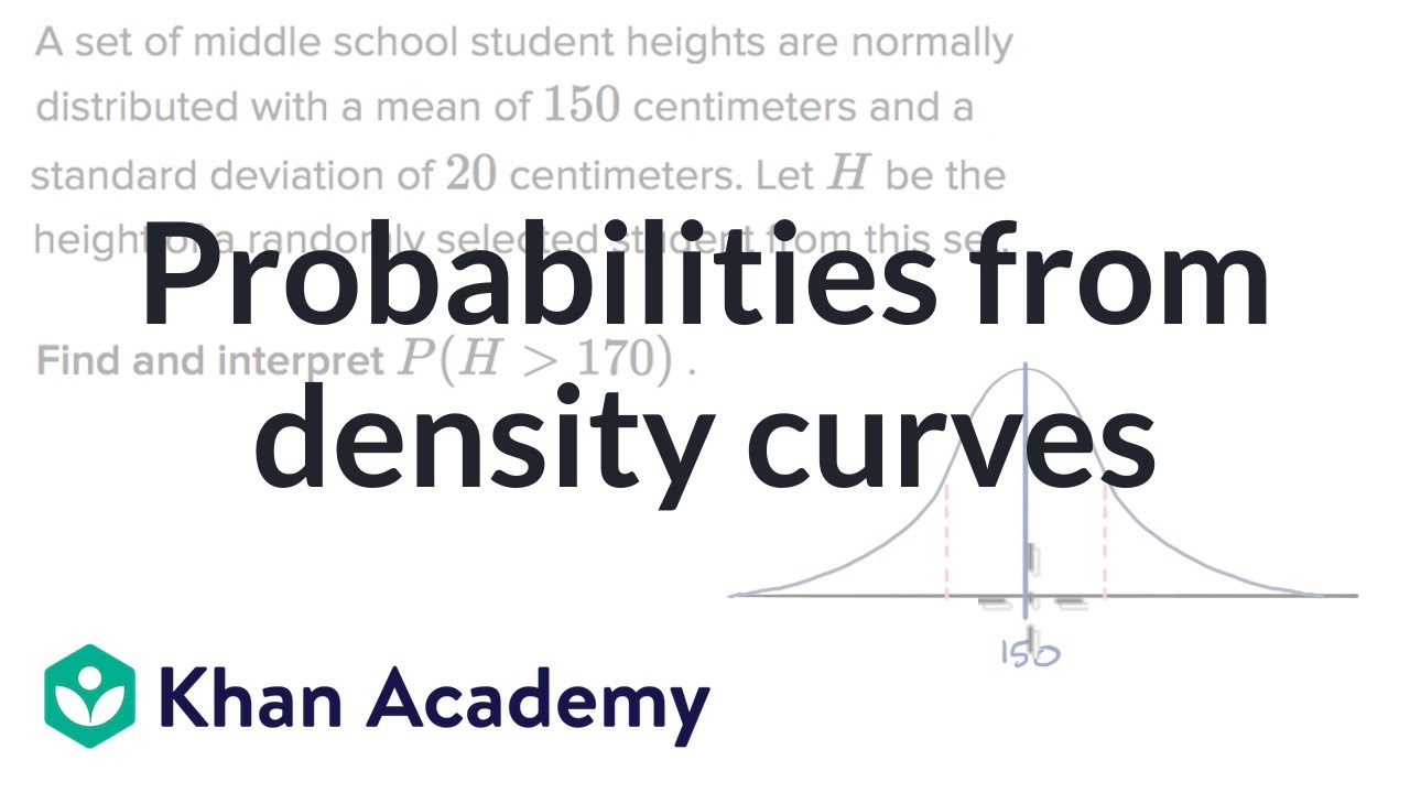
Probabilities from density curves | Random variables | AP Statistics | Khan Academy
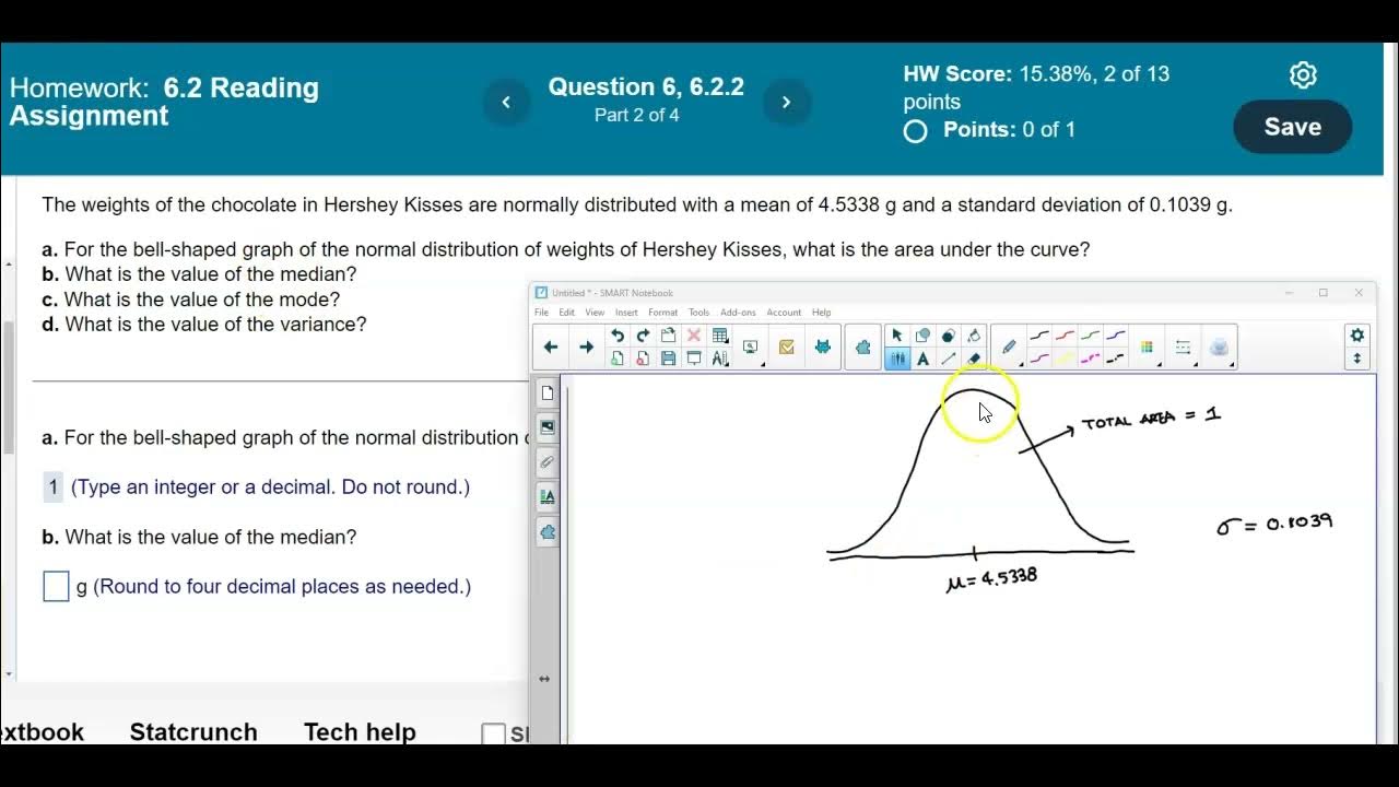
Math 14 6.2.2 What is the area under the curve & values of the median, mode & variance?
The Main Ideas behind Probability Distributions
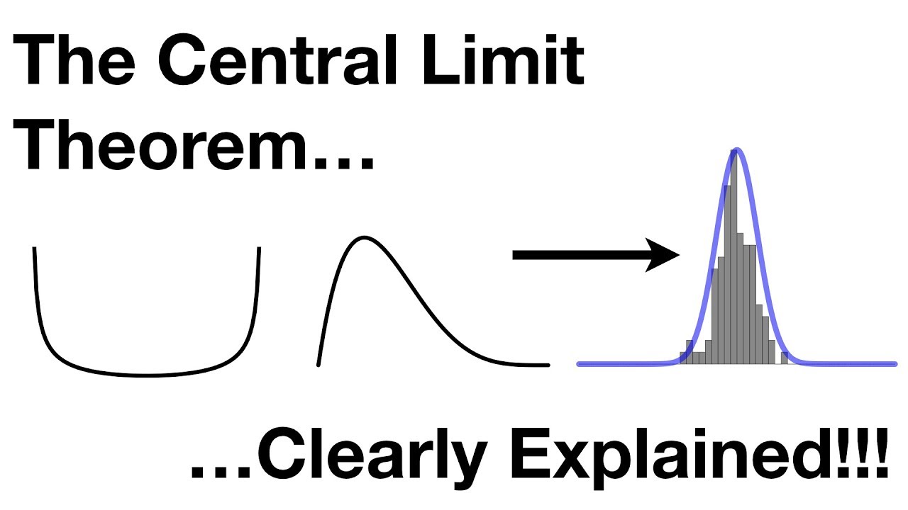
The Central Limit Theorem, Clearly Explained!!!
Hypothesis Testing Explained | Statistics Tutorial | MarinStatsLectures
5.0 / 5 (0 votes)
Thanks for rating: