GCSE Physics - Velocity Time Graphs #54
TLDRThis educational video delves into velocity time graphs, emphasizing their importance in understanding an object's velocity changes over time. It highlights the distinction between velocity and distance time graphs, explaining that the gradient on a velocity time graph represents acceleration. The video instructs on calculating constant acceleration, deceleration, and velocity during flat sections, and introduces a method for estimating the distance traveled by calculating the area under the curve. It concludes with a practical example of approximating the area under a curve for distance calculation.
Takeaways
- 📈 Velocity-time graphs display an object's velocity changes over time, with velocity on the y-axis and time on the x-axis.
- 🔄 It's crucial to distinguish between distance-time and velocity-time graphs, as they look similar but represent different physical quantities.
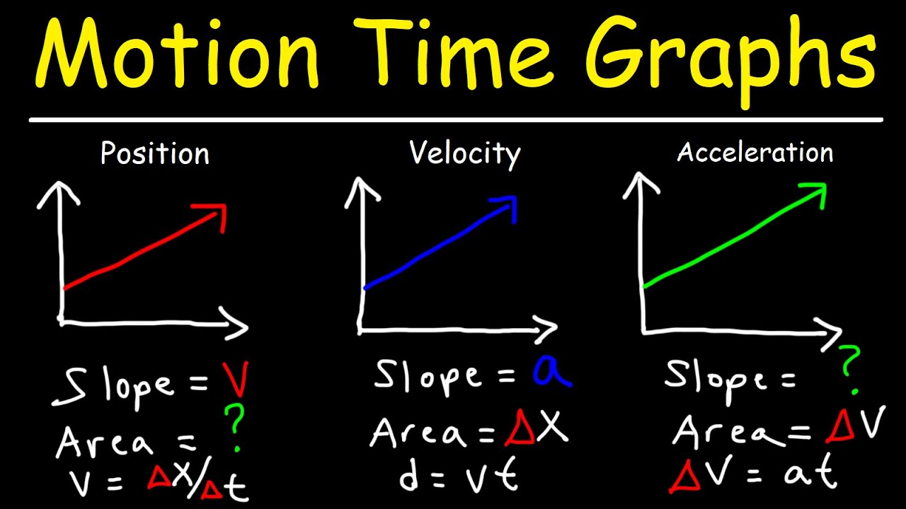
- 🧠 Understanding the gradient of the curve on a velocity-time graph is essential, as it represents the acceleration of the object.
- 🚀 A constant positive gradient indicates constant acceleration, while a constant negative gradient signifies constant deceleration.
- 🔢 To calculate acceleration or deceleration, use the formula change in velocity over change in time, which is the same as the definition of acceleration.
- 🏃 Flat sections of the curve with a gradient of 0 indicate no acceleration, meaning the velocity is constant.
- 📏 During constant velocity sections, the y-axis value directly gives the velocity of the object.
- 📈 When the curve steepens, it indicates that the rate of acceleration is increasing.
- 📐 The distance traveled can be found by calculating the area under the curve, with different shapes having their respective area formulas.
- 📊 For estimating the area under curved parts of the graph, use a grid system on the graph background and count the squares, including partial squares, to approximate the area.
- 🎓 Remember that even though area is usually in square meters, distance traveled is represented in meters, not squared meters.
Q & A
What is the main focus of the video?
-The main focus of the video is on velocity time graphs and how they differ from distance time graphs.
How can one differentiate between a velocity time graph and a distance time graph?
-A velocity time graph has velocity on the y-axis and time on the x-axis, whereas a distance time graph has distance on the y-axis and time on the x-axis.
What does the gradient of a velocity time graph represent?
-The gradient of a velocity time graph represents the acceleration of the object.
What type of acceleration is experienced when the curve has a constant positive gradient?
-When the curve has a constant positive gradient, the object is experiencing constant acceleration.
What happens when the curve has a constant negative gradient in a velocity time graph?
-When the curve has a constant negative gradient, there is constant deceleration.
How is acceleration calculated on a velocity time graph?
-Acceleration is calculated by finding the change in velocity divided by the change in time at any given point on the graph.
What does a flat section of the curve in a velocity time graph indicate?
-A flat section of the curve indicates that the object is not accelerating, meaning its velocity is constant.
How can one determine the velocity during constant velocity stages?
-During constant velocity stages, one can determine the velocity by looking at the y-axis value at that particular time.
What does the gradient increasing indicate in the context of a velocity time graph?
-If the gradient is increasing, it means that the rate of acceleration is also increasing.
How is the distance traveled calculated on a velocity time graph?
-The distance traveled is calculated by finding the area under the curve, which can be done by breaking it down into simple shapes like triangles and rectangles and calculating their areas.
Why do we leave the distance traveled answer in meters instead of converting it to meters squared?
-We leave the answer in meters because we are calculating the actual distance traveled, not an area.
How can one estimate the area under curved parts of the graph?
-One can estimate the area under curved parts by counting the number of squares under that section of the graph and combining them into full squares to get an approximate area.
Outlines
📊 Understanding Velocity Time Graphs
This paragraph introduces the concept of velocity time graphs, which illustrate the variation of an object's velocity over time. It emphasizes the importance of distinguishing between distance-time and velocity-time graphs, as they can appear similar but represent different physical quantities. The paragraph explains that the gradient of the curve on a velocity-time graph represents acceleration, with positive gradients indicating constant acceleration and negative gradients indicating constant deceleration. The method for calculating acceleration or deceleration is provided, using the formula change in velocity over change in time. Additionally, the paragraph describes how to determine the constant velocity during flat sections of the graph and the increasing rate of acceleration when the curve steepens. The process of calculating the distance traveled by finding the area under the curve is also detailed, with examples provided for both triangular and rectangular areas.
👋 Conclusion and Future Lessons
The paragraph concludes the video by summarizing the main points discussed about velocity-time graphs and their practical applications in understanding an object's motion. It also encourages viewers to share the video with friends and teachers, creating a sense of community and continued learning. The speaker expresses a friendly farewell, indicating that more information will be covered in the next video, thus inviting viewers to stay tuned for future content.
Mindmap
Keywords
💡Distance-time graphs
💡Velocity-time graphs
💡Gradient
💡Acceleration
💡Deceleration
💡Constant velocity
💡Area under the curve
💡Curve steepness
💡Calculating distance
💡Acceleration calculation example
Highlights
The video focuses on velocity time graphs, which are essential for understanding how an object's velocity changes over time. (Start Time: 0s)
Velocity time graphs can be easily confused with distance time graphs, so it's crucial to double-check which one you're analyzing. (Start Time: 10s)
The gradient of the curve on a velocity time graph represents acceleration, providing valuable insights into an object's motion. (Start Time: 20s)
A constant positive gradient indicates a constant acceleration, while a constant negative gradient signifies constant deceleration. (Start Time: 30s)
The acceleration can be calculated using the formula change in velocity over change in time. (Start Time: 40s)
Flat sections of the curve have a gradient of 0, indicating no acceleration and a constant velocity. (Start Time: 50s)
The velocity during constant velocity stages can be found by looking at the y-axis value. (Start Time: 1m)
If the curve gets steeper, it means the rate of acceleration is increasing. (Start Time: 1m 10s)
The total distance traveled can be found by calculating the area under the curve. (Start Time: 1m 20s)
For straight-line sections, the area can be calculated as a simple rectangle, and for curved sections, estimation is required. (Start Time: 1m 30s)
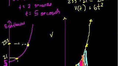
In the example provided, the distance traveled in the first four seconds is calculated by breaking the area into a triangle and a rectangle. (Start Time: 1m 40s)
The area of the triangle is calculated as 0.5 times base times height, resulting in 3 meters. (Start Time: 1m 50s)
The area of the rectangle is calculated as base times height, resulting in 6 meters. (Start Time: 2m)
The total distance traveled in the first four seconds is 9 meters, calculated by adding the areas of the triangle and rectangle. (Start Time: 2m 10s)
When calculating the area under curved parts of the graph, a grid can be used to estimate the distance traveled. (Start Time: 2m 20s)
For the curved section, the total estimated distance traveled is around 8 meters, by counting full and partially filled squares. (Start Time: 2m 30s)
Although area is usually given in square meters, the distance traveled is left in meters for simplicity. (Start Time: 2m 40s)
The video concludes with an encouragement to share the content with friends and teachers, highlighting the educational value of the material. (Start Time: 2m 50s)
Transcripts
Browse More Related Video

High School Physics: Graphing Motion
Velocity Time Graphs, Acceleration & Position Time Graphs - Physics

GCSE Physics Revision "Acceleration"

Acceleration vs. time graphs | One-dimensional motion | Physics | Khan Academy
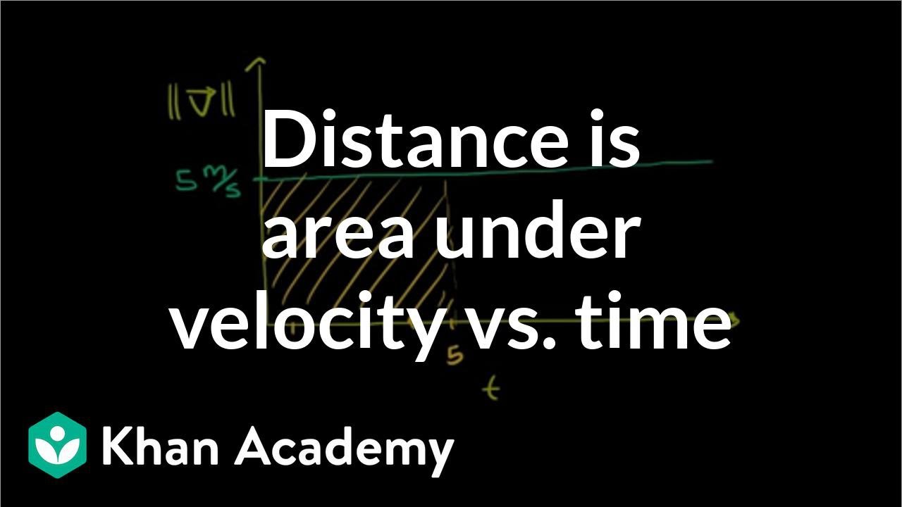
Why distance is area under velocity-time line | Physics | Khan Academy
Definite Integrals (area under a curve) (part III)
5.0 / 5 (0 votes)
Thanks for rating: