Graphing Piecewise Functions - Precalculus
TLDRThis tutorial delves into graphing piecewise functions, illustrating how to combine different segments based on the domain of the variable. Starting with a basic example, the video demonstrates graphing a linear function for x < 0 and a horizontal line for x ≥ 0. It proceeds to more complex examples, showing how to handle different expressions and intervals, including open and closed circles to indicate inclusion or exclusion of certain points. The tutorial emphasizes step-by-step plotting and understanding the mathematical behavior of piecewise functions, ultimately guiding viewers to visualize and comprehend the graphs of various piecewise functions.
Takeaways
- 📈 Piecewise functions are composed of different segments with distinct expressions for different ranges of the domain.
- 🌟 The graph of a piecewise function is a combination of the graphs of its individual segments.
- 📌 For the function f(x) = x when x < 0 and f(x) = 5 when x ≥ 0, the graph consists of a line with a slope of one (y=x) for negative x values and a horizontal line at y=5 for non-negative x values.
- 🔺 Use open circles to indicate that a point is not included in the function's domain, and closed circles for points that are included.
- 🔄 When graphing, it's important to consider the slope and y-intercept for linear segments and the shape for non-linear segments.
- 📊 For the function f(x) = 2 when x < 1, f(x) = x + 3 when 1 < x < 2, and f(x) = 5 when x ≥ 2, the graph starts as a horizontal line at y=2, transitions to a line with a slope of one, and ends with a horizontal line at y=5.
- 🔼 The y-intercept is the point where the graph crosses the y-axis, and it's found by setting x to zero in the function's expression.
- 🔄 For the function f(x) = 2x + 1 when x < 1, f(x) = 1 when x = 1, and f(x) = -x^2 when x > 1, the graph includes a line with a slope of two, a single point at (1,1), and a downward-opening parabola.
- 🔢 The graph of a piecewise function must reflect the correct domain restrictions, such as including or excluding certain x values.
- 📈 For the function f(x) = 3x + 4 when x < 0, f(x) = 2 when x = 0, and f(x) = √x when x > 1, the graph starts as a line with a y-intercept at (0,4), has a single point at (0,2), and transitions to an increasing function that rises more slowly as x increases.
- 🔄 When x < 0, the graph of 1/x is negative, and when x ≥ 0, it's positive. The function's graph includes a horizontal line at y=3 for 0 < x < 3 and a linearly decreasing function for x ≥ 3.
Q & A
What is the definition of a piecewise function?
-A piecewise function is a mathematical function that is defined by multiple sub-functions, each applicable within a specific interval or set of inputs. The function changes its formula or rule depending on the range of the independent variable.
How is the graph of the function f(x) = x for x < 0 represented?
-The graph of the function f(x) = x for x < 0 is represented as a straight line with a slope of one, rising at a 45-degree angle. This line extends from the origin (0,0) to the left, not including the point (0,0), and is marked with an open circle at the origin.
What does the graph of f(x) = 5 for x ≥ 0 look like?
-The graph of f(x) = 5 for x ≥ 0 is a horizontal line at y = 5, including the point (0,5) since the function is defined at x = 0. This line extends infinitely to the right and is marked with a closed circle at the point (0,5).
How do you combine the two graphs for the function f(x) = x for x < 0 and f(x) = 5 for x ≥ 0?
-To combine the two graphs, you plot the left side of the graph for y = x (rising line) up to but not including the origin, and then connect it to the right side of the graph for y = 5 (horizontal line) starting at the origin. This creates a corner or step at the point (0,5) where the two lines meet.
What is the second example function given in the script, and how is it graphed?
-The second example function is f(x) = 2 when x < 1, and f(x) = x + 3 when x ≥ 1. The graph starts as a horizontal line at y = 2 for x < 1 (with an open circle at (1,2) since it does not include x = 1), and then transitions to a line with a slope of 1 and a y-intercept of 3 for x ≥ 1.
How do you determine if a point should be marked with an open or closed circle on a piecewise function graph?
-A point is marked with an open circle if the value is not included in the function's domain for that interval, and with a closed circle if the value is included. This indicates whether the function is defined at that particular point.
What is the third example function discussed in the script, and what are its key features?
-The third example function is f(x) = 2x + 1 when x < 1, f(x) = 1 when x = 1, and f(x) = -x^2 when x > 1. It starts with a line of slope 2 and y-intercept 1 for x < 1, has a single point (1,1) at x = 1, and then transitions to a downward-opening parabola with a vertex at (0,0) for x > 1.
How does the graph of the function f(x) = 3x + 4 for x < 0 change when x = 0?
-The graph of f(x) = 3x + 4 for x < 0 is a straight line with a slope of 3 and a y-intercept at (0,4). When x = 0, the graph has a closed circle at the point (0,4), indicating the function's value at the origin is included in the domain.
What is the function f(x) = √x for x > 1, and how does its graph behave?
-The function f(x) = √x for x > 1 represents the square root of x. Its graph is an increasing function that rises more slowly as x increases, starting at (1,1) and continuing to rise but at a decreasing rate.
In the final example, how does the function f(x) change when x ≥ 3?
-In the final example, when x ≥ 3, the function f(x) is defined as f(x) = -x + 5. The graph starts at (3,2) with a closed circle, indicating the function is defined at x = 3, and then decreases as x increases, following a straight line with a slope of -1.
What is the x-intercept of the function f(x) = -x + 5 for x ≥ 3?
-The x-intercept of the function f(x) = -x + 5 for x ≥ 3 is found by setting y to zero and solving for x. When x = 5, f(x) = -5 + 5 = 0, so the x-intercept is at the point (5,0).
How can you ensure that you graph a piecewise function correctly?
-To graph a piecewise function correctly, take your time and graph it step by step, plotting the relevant parts of the function according to their respective intervals. Pay attention to the open or closed circles at key points to indicate whether the function includes those points in its domain.
Outlines
📊 Graphing Piecewise Functions - Introduction and First Example
This paragraph introduces the concept of graphing piecewise functions, starting with a specific example. The function in focus is f(x) = x for x < 0 and f(x) = 5 for x ≥ 0. The explanation details how to graph these two segments separately: the first as a straight line with a slope of one (45-degree angle), and the second as a horizontal line at y = 5. It then describes how to combine these two parts to form the piecewise function graph, emphasizing the use of open and closed circles at particular points to indicate inclusion or exclusion of those points.
📈 Second and Third Piecewise Function Examples
This paragraph presents two additional piecewise function examples. The first example is f(x) = 2 for x < 1 and f(x) = x + 3 for x ≥ 1, highlighting the use of open circles at points of discontinuity and the creation of a graph with a y-intercept of 3 and a slope of 1. The second example discusses f(x) = 2x + 1 for x < 1, f(x) = 1 for x = 1, and f(x) = -x^2 for x > 1. It covers the graphing of a linear function with a slope of 2 and a y-intercept of 1, a constant horizontal line, and a downward-opening parabola. Each segment is detailed, including the points and the transitions between them.
📉 Advanced Piecewise Function Examples and Techniques
The final paragraph delves into more complex piecewise functions, starting with f(x) = 3x + 4 for x < 0, f(x) = 2 for x = 0, and f(x) = √x for x > 0. It explains how to graph a linear function with a y-intercept at (0,4), a constant value at x = 0, and a square root function with an open circle at x = 1. The paragraph then presents the last example of f(x) = 1/x for x < 0, f(x) = 3 for 0 ≤ x < 3, and f(x) = -x + 5 for x ≥ 3. It describes the graphing process, including the negative reciprocal function, a horizontal line, and a linear function with a negative slope. The summary emphasizes understanding the behavior of the function at the breakpoints and the visual representation of the piecewise function.
Mindmap
Keywords
💡Piecewise Functions
💡Graphing
💡Slope
💡Domain
💡Y-intercept
💡Parabola
💡X-intercept
💡Closed Circle
💡Open Circle
💡Square Root Function
💡One Over X
Highlights
The tutorial focuses on graphing piecewise functions, starting with a specific example of a function defined differently for x < 0 and x ≥ 0.
The first function, f(x) = x for x < 0, is represented by a straight line with a slope of one, rising at a 45-degree angle.
The second part of the example function, f(x) = 5 for x ≥ 0, is a horizontal line at y = 5.
When graphing piecewise functions, the left side of the graph (y = x) is used for x < 0, and the right side (y = 5) for x ≥ 0, combining both parts.
For the second example, f(x) = 2 for x < 1 and f(x) = x + 3 for x > 2, the graph includes a horizontal line at y = 2 for x < 1 and a line with a slope of 1 and y-intercept of 3 for x > 2.
An open circle is used at points where the function does not include the value (e.g., x = 1), and a closed circle where it does (e.g., x = 0).
The third example involves a function with a linear part (2x + 1 for x < 1), a single point (f(1) = 3), and a parabolic part (-x^2 for x > 1).
The linear part of the third example has a slope of 2 and a y-intercept of 1, and is only plotted for x < 1.
The parabolic part of the third example opens downward, with the function not including x = 1, and showing a curved shape.
In the fourth example, the function is a linear equation (3x + 4 for x < 0), a constant (f(x) = 2 for x = 0), and a square root function (sqrt(x) for x > 1).
The linear part of the fourth example has a y-intercept at (0, 4) and is only graphed for x < 0.
The constant part of the fourth example is represented by a single point at (0, 2) with a closed circle, as it includes x = 0.
The square root function part of the fourth example increases at a decreasing rate and is represented by an open circle at points where it does not include the x value.
The last example involves a function with a reciprocal part (1/x for x < 0), a constant part (f(x) = 3 for 0 ≤ x < 3), and a linear part with a negative slope (-x + 5 for x ≥ 3).
The reciprocal part of the last example has a positive and negative section, with only the negative section (x < 0) being graphed.
The linear part of the last example has a slope of -1, with a zero x-intercept, and shows a downward trend as x increases.
The process of graphing piecewise functions involves understanding the domain restrictions and the behavior of each part of the function.
Transcripts
Browse More Related Video
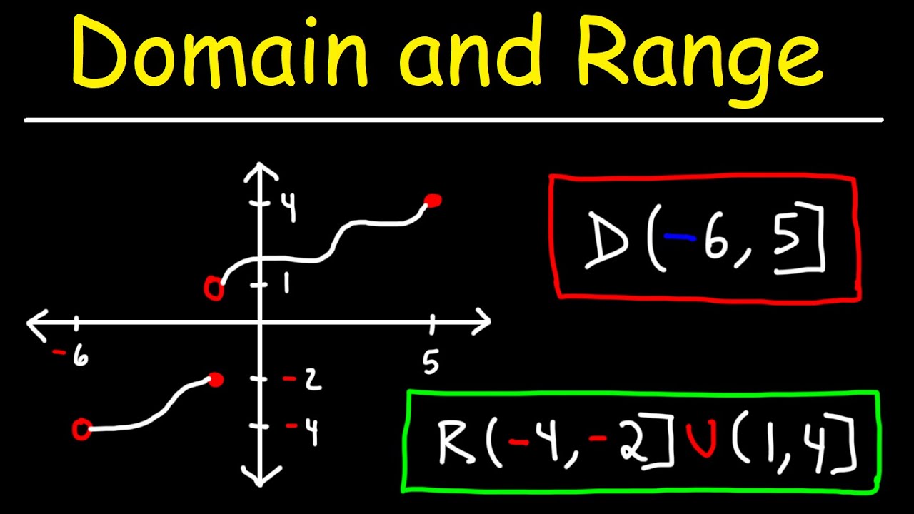
Domain and Range of a Function From a Graph
Piecewise Functions
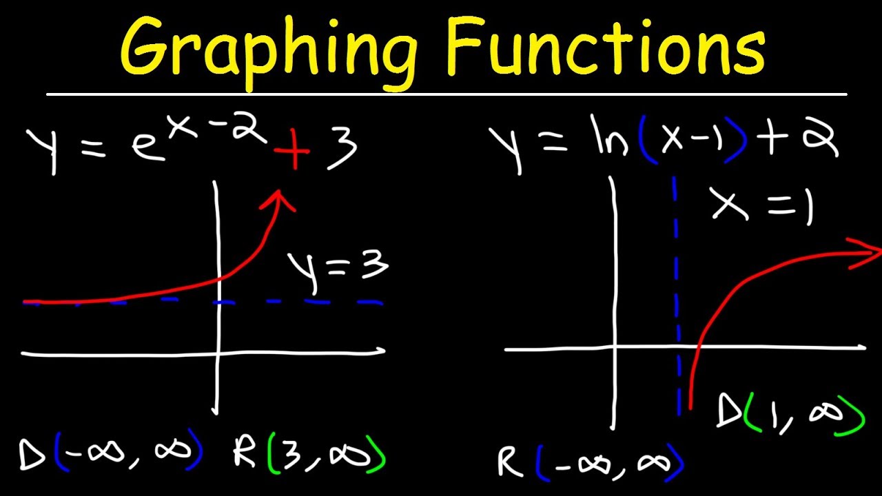
Graphing Natural logarithmic functions and Exponential Functions

Evaluating Piecewise Functions | PreCalculus
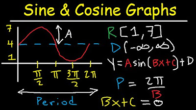
Graphing Sine and Cosine Trig Functions With Transformations, Phase Shifts, Period - Domain & Range

Definite integral of piecewise function | AP Calculus AB | Khan Academy
5.0 / 5 (0 votes)
Thanks for rating: