Intermediate value theorem example | Existence theorems | AP Calculus AB | Khan Academy
TLDRThe video script discusses the Intermediate Value Theorem, a fundamental concept in calculus, which states that a continuous function on a closed interval will take on every value between the function's values at the interval's endpoints. Using the given function F, defined on the interval from negative two to one with F(-2) = 3 and F(1) = 6, the video explains that there must exist at least one value C within the interval for which F(C) equals four, as four lies between three and six. The explanation is supported by visual reasoning, illustrating the continuous nature of the function and its implications on the values it assumes.
Takeaways
- 📈 The Intermediate Value Theorem applies to continuous functions on closed intervals.
- 🔢 A continuous function on a closed interval will take every value between the function's values at the interval's endpoints.
- 📌 The function F is given with F(-2) = 3 and F(1) = 6.
- 🎯 The theorem guarantees that for any value L between 3 and 6, there exists at least one C in the interval [-2, 1] such that F(C) = L.
- ✏️ The value of C must be within the interval, and L must be between the function's endpoints' values.
- 🚫 The theorem does not guarantee that the function will take on values outside the range of the endpoints' values.
- 🌐 The concept can be visualized by plotting the function's graph and ensuring it is continuous without lifting the pen.
- 📍 The graph of the function must include the points (-2, 3) and (1, 6).
- 🔄 The function can take on multiple values of four (4) within the interval [-2, 1], as long as it is continuous.
- 🥇 The key example from the script is that F(C) = 4 for some C in the interval [-2, 1], since 4 is between 3 and 6.
- 🧩 The theorem is a fundamental concept in calculus and helps in understanding the behavior of continuous functions.
Q & A
What is the Intermediate Value Theorem and how does it apply to the given scenario?
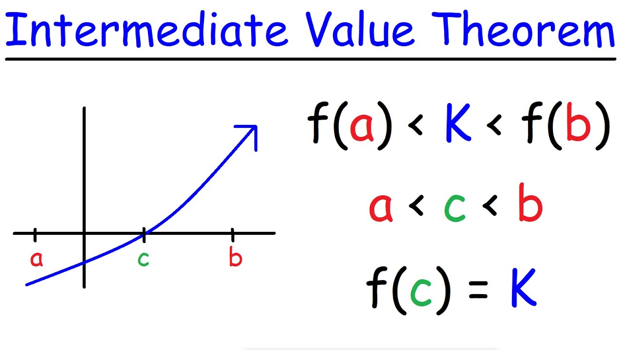
-The Intermediate Value Theorem (IVT) states that if a function is continuous on a closed interval, then it must take on every value between the values at the endpoints of the interval. In the given scenario, since F is a continuous function on the closed interval from -2 to 1 with F(-2) equal to 3 and F(1) equal to 6, the IVT guarantees that for any value L between 3 and 6, there exists at least one c in the interval such that F(c) = L.
What are the conditions for the Intermediate Value Theorem to hold?
-The Intermediate Value Theorem holds if the function is continuous on a closed interval. In the provided script, the function F is continuous on the closed interval from -2 to 1, which satisfies the conditions for the IVT to apply.
What is the significance of the function values at the endpoints of the interval in the context of the IVT?
-The function values at the endpoints of the interval are crucial because they define the range of possible values the function can take within the interval. According to the IVT, the function must take on every value between these endpoint values at least once within the closed interval.
Why is it important that the interval in the IVT is closed?
-A closed interval includes its endpoints, which means the function is evaluated at those points. This is important for the IVT because it ensures that the function has the opportunity to take on every value between the endpoint values, including the endpoints themselves.
How does the IVT help in determining the existence of roots for a function?
-The IVT can be used to verify the existence of a root (or zero) of a function within a given interval. If the function values at the endpoints of the interval have opposite signs (one is positive and the other is negative), then by the IVT, there must be at least one root in that interval where the function crosses the x-axis.
What does the IVT tell us about the function's behavior between the endpoints?
-The IVT tells us that the function is guaranteed to take on every value between the function values at the endpoints within a closed interval. This means that if the function is continuous, it will not 'skip' any values in that range without first lifting the pencil from the paper (a visual way to think about continuity).
How can we visualize the IVT in the context of the given function F?
-We can visualize the IVT by plotting the known function values at the endpoints on the y-axis (F(-2) = 3 and F(1) = 6) and then drawing a continuous curve that includes these points. This curve must pass through every value between 3 and 6 at least once, as it cannot lift off the paper within the interval.
What is the role of the value L in the IVT?
-The value L represents any number between the function values at the endpoints of the interval. The IVT states that there exists at least one value c within the interval such that F(c) = L. This demonstrates the function's ability to take on a wide range of values within the interval due to its continuity.
Why is it incorrect to say that F(c) can be zero for some c between -2 and 1, according to the IVT?
-It is incorrect because the IVT only guarantees that the function will take on values between the function values at the endpoints of the interval. Since zero is not between 3 and 6 (the values of F at the endpoints), the IVT does not ensure that F(c) will be zero for any c in the interval.
How does the IVT relate to the concept of continuity in calculus?
-The IVT is a direct consequence of the definition of continuity. A continuous function is one whose graph can be drawn without lifting the pencil, which implies that it must take on every value between its values at the endpoints of a closed interval. The IVT is essentially a formal statement of this property of continuous functions.
What is the significance of the IVT in solving real-world problems?
-The IVT is significant in real-world problems because it provides a mathematical guarantee that certain conditions will be met within a given range. For example, in engineering, it can be used to ensure that a system will reach a desired state if it is continuously variable and the endpoints represent the initial and desired states.
Outlines
📚 Introduction to the Intermediate Value Theorem
This paragraph introduces the Intermediate Value Theorem within the context of a continuous function, F, on a closed interval from negative two to one. The theorem is explained as guaranteeing that the function will take on every value between the given endpoints' values, which in this case are three and six. The explanation includes a discussion on the implications of the theorem, emphasizing the necessity for the function to take on any value within the specified range, using the example of the value four to illustrate this point. The paragraph also encourages viewers to refer to a video on the theorem for a deeper understanding and concludes with a visual representation of the theorem's concept.
🎨 Visualizing the Continuous Function and its Values
In this paragraph, the speaker further elaborates on the concept of a continuous function by visualizing it on a graph. The speaker explains that since the function is continuous on the closed interval from negative two to one, it must take on every value between the endpoints' values, which are three and six. The speaker uses the value four as an example and illustrates how the function could potentially take on this value at multiple points within the interval. The paragraph also discusses alternative ways the function could be visualized, including as a straight line, and highlights that the specific shape of the function is not known, only that it must satisfy the conditions of the Intermediate Value Theorem within the given interval.
Mindmap
Keywords
💡Continuous function
💡Intermediate Value Theorem
💡Closed interval
💡Value of the function
💡Endpoints
💡Interval
💡Graph
💡Y-axis
💡X-axis
💡Plotting points
💡Value between three and six
Highlights
The Intermediate Value Theorem is discussed in the context of a continuous function on a closed interval.
The function F is defined on the closed interval from negative two to one, with specific values at the endpoints.
F of negative two is equal to three, and F of one is equal to six, providing boundary conditions for the theorem's application.
The theorem ensures that for any value L between the function's endpoints, there exists at least one C in the interval such that F of C equals L.
The theorem's applicability is confirmed by the function's continuity on the given closed interval.
A visual representation is suggested to better understand the theorem and the function's behavior.
The function must take on every value between the endpoint values, which in this case are three and six.
The example given is F of C equals four, which is a valid case since four is between three and six.
The importance of the value L being between the endpoint values is emphasized for the theorem to hold true.
The function's graph is described as continuous, meaning it cannot have gaps or jumps within the interval.
The graph of the function includes the points given by the boundary conditions and must be continuous between them.
The visual representation shows that the function takes on every value between three and six, satisfying the theorem's condition.
Multiple C values within the interval may satisfy the theorem, as the function could cross the value line multiple times.
The discussion includes the possibility of drawing the function's graph in various ways, all satisfying the theorem.
The example of the function being a straight line is provided, showing one way it could satisfy the theorem.
The theorem's practical application is demonstrated through the analysis of the function's behavior on the given interval.
The transcript concludes with the assertion that the function must take on the value four for at least one C in the interval, confirming the theorem's prediction.
Transcripts
Browse More Related Video
How to show that a solution exists to a functions using IVT
Intermediate Value Theorem
Calculus 1 Lecture 3.2: A BRIEF Discussion of Rolle's Theorem and Mean-Value Theorem.
Intermediate value theorem to prove a root in an interval (KristaKingMath)

Using the Intermediate Value Theorem Examples
Justification with the intermediate value theorem: table | AP Calculus AB | Khan Academy
5.0 / 5 (0 votes)
Thanks for rating: