Learn Statistical Regression in 40 mins! My best video ever. Legit.
TLDRIn this refreshingly updated video, Justin Zeltzer of Zedstatistics embarks on a mission to demystify regression analysis for both beginners and those seeking a foundational understanding. Spanning a comprehensive 40-minute journey, Justin dives deep into the objectives behind regression, explaining its essence through intuitive examples like ice cream sales influenced by variables like temperature and rainfall. He navigates through the population regression equation, sample regression lines, and the intricacies of SST, SSR, and SSE. The video further explores the significance of r-squared and adjusted r-squared values, providing insights into degrees of freedom. By the end, viewers are promised a zero-to-hero mastery of regression, making complex statistical concepts accessible and engaging.
Takeaways
- 📚 Justin Zeltzer updates his most popular video on regression to provide a comprehensive, 40-minute tutorial aimed at beginners or those seeking a solid foundation in the topic.
- 📈 The video starts with the basics of regression, explaining its objectives and giving viewers an intuitive understanding of what regression is all about.
- 📝 Discusses the population regression equation and the sample regression line, highlighting how data is incorporated to create a regression line and estimate coefficients.
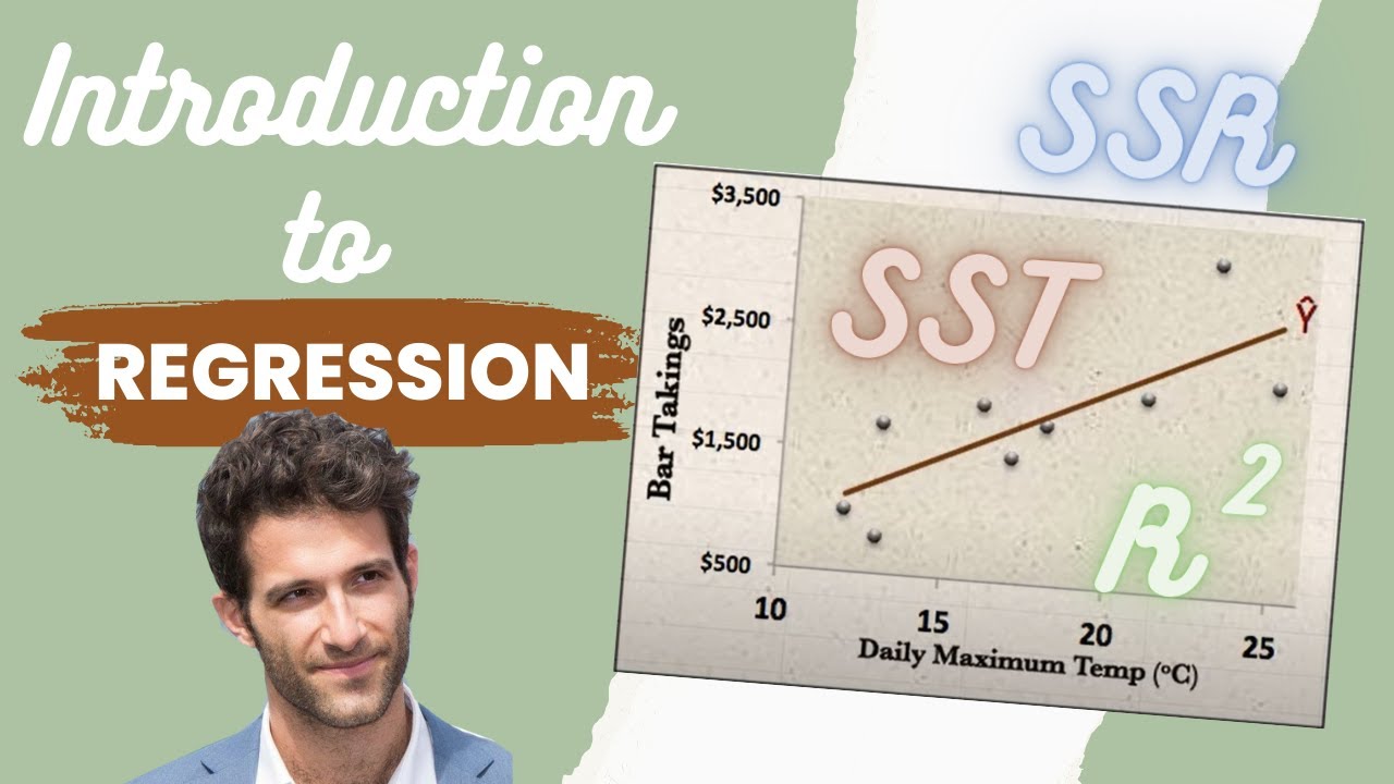
- 🔧 Delves into SST, SSR, and SSE - the mathematical 'nuts and bolts' behind creating a regression line, and clarifies common confusions regarding their terminology.
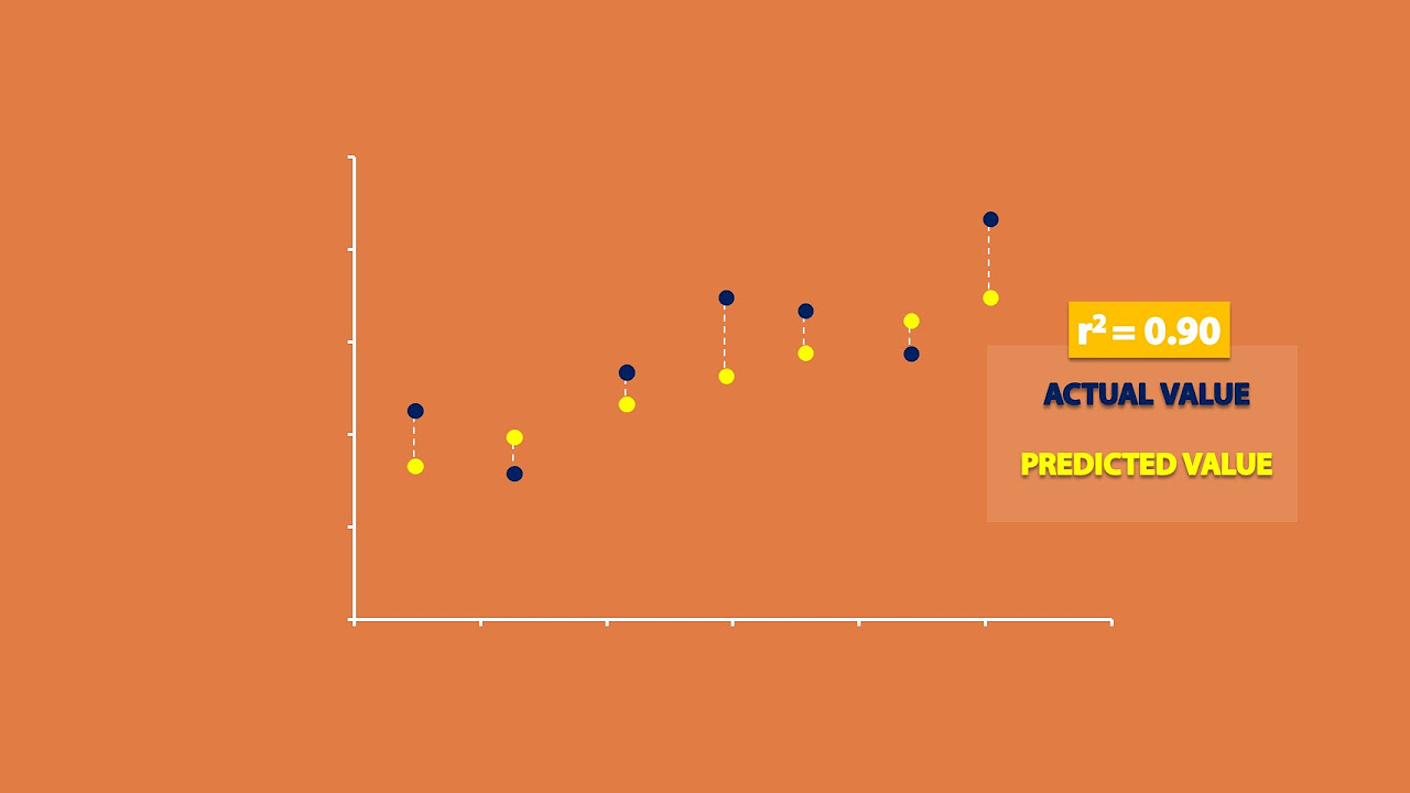
- 🛠 Introduces the concept of R-squared as a measure of the strength of a regression, helping viewers understand the proportion of variance in the dependent variable that is predictable from the independent variable.
- 🔎 Covers the topic of adjusted R-squared and degrees of freedom, offering a unique explanation that adds depth to the viewers' understanding of these concepts.
- 📊 Provides practical examples, like ice cream sales prediction using temperature, rainfall, and school holidays as variables, to illustrate regression analysis in action.
- 🚧 Warns against the pitfalls of adding too many explanatory variables to a model, which can artificially inflate R-squared values without actually improving the model's predictive power.
- 💎 Highlights the importance of using adjusted R-squared for model comparison, especially when models have different numbers of explanatory variables.
- 📍 Promotes a holistic approach to understanding regression, encouraging viewers to appreciate both the theory behind regression analysis and its practical applications.
Q & A
What is the main purpose of the video by Justin Zeltzer?
-The main purpose of the video is to provide a comprehensive and updated explanation on the topic of regression, aimed at both newcomers to the topic and those seeking a solid foundation in understanding it.
How does Justin Zeltzer plan to structure the video content?
-Justin plans to structure the video by starting with the objectives behind regression, discussing the population regression equation, and then moving on to the sample regression line. He will also cover the concepts of SST, SSR, and SSE, the measure of the strength of a regression through r-squared, and the topics of adjusted r-squared and degrees of freedom.
What is the definition of regression provided in the video?
-Regression is defined as a means of exploring the variation in some quantity, separating that variation into what can be explained and what is unexplained.
What is the role of the independent variable (X) and the dependent variable (Y) in the population regression equation?
-In the population regression equation, the independent variable (X) is the variable that is used to explain or predict the dependent variable (Y). The dependent variable (Y) is the outcome that the model is trying to predict or explain based on the independent variable.
What is the significance of the coefficients in the population regression equation?
-The coefficients in the population regression equation, beta naught (β₀) and beta one (β₁), represent the intercept and slope of the regression line, respectively. They quantify the relationship between the independent variable (X) and the dependent variable (Y).
How does the sample regression line differ from the population regression equation?
-The sample regression line differs from the population regression equation in that it uses estimated values (beta naught hat and beta one hat) based on sample data to create the best-fit line through the data points, and it does not include an error term.
What is the process of creating a sample regression line?
-The process of creating a sample regression line involves using a dataset to find the best-fit line through the data points. This line represents the best estimate for the relationship between the independent and dependent variables.
What is the goal of minimizing the sum of squared error terms in regression?
-Minimizing the sum of squared error terms aims to find the line of best fit that has the smallest possible distance between the observed data points and the predicted values on the line, thus providing the best model fit for the data.
What is the role of the error term in the sample regression line equation?
-The error term in the sample regression line equation represents the difference between the actual observed value of Y and the predicted value of Y (y hat) for each individual observation.
What does the adjusted R-squared value indicate?
-The adjusted R-squared value adjusts the R-squared for the number of explanatory variables in the model and the number of observations, providing a more accurate measure of how well the model explains the variation in the dependent variable, especially when comparing models with different numbers of predictors.
Why is it important to consider degrees of freedom when adding explanatory variables to a regression model?
-Considering degrees of freedom is important because it reflects the model's ability to show error. As more explanatory variables are added, the degrees of freedom decrease, which can lead to overfitting and a less accurate representation of the model's performance, as the model loses the ability to account for variability in the data.
Outlines
📊 Introduction to the New Regression Video
Justin Zeltzer introduces a revamped version of his popular regression video from a decade ago, acknowledging the original's success despite its shortcomings. The new 40-minute guide aims to provide a comprehensive foundation on regression for both newcomers and those seeking a refresher. The video promises valuable insights, starting with the basics of regression, exploring its objectives, equations, and key mathematical concepts like SST, SSR, SSE, R squared, and adjusted R squared. Justin encourages viewers to engage with the content, promising a journey from zero to hero in understanding regression.
🔍 Understanding Regression: Objectives and Basics
The video delves into the objectives behind regression, explaining it as a method to explore variation in quantities by separating it into explained and unexplained components. Justin uses the example of ice cream sales, influenced by daily temperature, rainfall, and school holidays, to illustrate how regression can quantify the variation in sales. This section establishes the foundation of regression, emphasizing its role in distinguishing between the explained and unexplained variation, setting the stage for deeper exploration of regression equations and data analysis.
📈 The Population Regression Equation and Data Incorporation
Justin introduces the population regression equation, emphasizing the relationship between dependent and independent variables, and the role of coefficients and error terms. He simplifies the concept by comparing it to the familiar linear equation from high school mathematics, highlighting the importance of estimating coefficients and quantifying error. The discussion transitions to incorporating actual data for creating a sample regression line, addressing the need for empirical evidence to estimate theoretical population regression parameters. This segment reinforces the significance of data in refining our understanding of regression models.
📉 Sample Regression Line and Error Term Exploration
Focusing on the sample regression line, Justin explains its derivation and the importance of the error term in capturing the deviation from predicted values. Through a practical example of ice cream sales, he illustrates how the line of best fit is determined by minimizing the sum of squared errors, introducing the concept of Ordinary Least Squares regression. This section emphasizes the analytical process behind regression analysis, demonstrating how theoretical concepts are applied to real-world data to identify the best-fitting regression line.
🔢 SSR, SSE, and SST: Breaking Down Regression Mathematics
Justin tackles the mathematical core of regression analysis by explaining SST, SSR, and SSE—key components that quantify total, explained, and unexplained variation, respectively. Using intuitive examples, he demonstrates how regression analysis separates total variation into components, providing insight into the extent to which independent variables explain the variation in the dependent variable. This explanation lays the groundwork for understanding the effectiveness and limitations of regression models in explaining real-world phenomena.
📚 Adjusted R Squared and Degrees of Freedom Explained
In the final sections, Justin addresses the concept of R squared and its limitations, leading to an introduction of adjusted R squared and degrees of freedom. He challenges viewers to think critically about the number of data points required for a meaningful regression analysis and the impact of adding explanatory variables on model accuracy. Through examples involving ice cream sales and various explanatory variables, including nonsensical ones like moon phases, he illustrates how adjusted R squared provides a more accurate reflection of a model's explanatory power, especially when dealing with multiple variables.
🎶 Conclusion and Invitation to Engage
The video concludes with an invitation for viewers to engage with the content by liking, commenting, and subscribing to the channel for future updates. Justin shares his journey from creating educational content to becoming a school teacher and hints at upcoming projects related to applying high school mathematics to real-world scenarios. This closing segment reinforces the video's educational value and encourages viewers to stay connected for more insightful content.
Mindmap
Keywords
💡Regression
💡Population Regression Equation
💡Sample Regression Line
💡Ordinary Least Squares (OLS)
💡SST, SSR, and SSE
💡R-squared
💡Adjusted R-squared
💡Degrees of Freedom
💡Error Term
💡Independent and Dependent Variables
Highlights
Justin Zeltzer introduces a new video on regression, aiming to provide a comprehensive understanding for newcomers and a solid foundation for those familiar with the topic.
The video promises to cover the essentials of regression, from the basics to advanced concepts like adjusted R-squared and degrees of freedom, in a 40-minute informative session.
Regression is defined as a method to explore variation in a quantity, separating it into explained and unexplained components.
The population regression equation is introduced, highlighting the relationship between the dependent variable (Y), the independent variable (X), and the error term.
The video explains the role of coefficients (beta naught and beta one) in estimating the linear relationship between Y and X in regression analysis.
The concept of the sample regression line is introduced, showing how it is derived from a dataset and how it differs from the population regression equation.
The process of creating the best-fit line using the method of least squares is discussed, emphasizing the minimization of the sum of squared error terms.
SSR (sum of squares due to regression) and SSE (sum of squares due to error) are explained, detailing how they quantify the explained and unexplained variance in the regression model.
The video clarifies the difference between r (correlation coefficient) and E (error term), noting that some textbooks may reverse these notations.
R-squared is introduced as a measure of the strength of a regression, representing the proportion of the variation in Y explained by X.
Adjusted R-squared is discussed, addressing its importance in adjusting for the number of explanatory variables and preventing overfitting in regression models.
Degrees of freedom in regression are explained, illustrating how they relate to the number of observations and explanatory variables, and their impact on the model's ability to show error.
The video addresses the potential pitfall of increasing R-squared by adding irrelevant variables, which can lead to overfitting and a false sense of model improvement.
Adjusted R-squared is presented as a more reliable measure for comparing models, as it accounts for the loss of degrees of freedom when additional variables are added.
Justin Zeltzer recommends a podcast called 'A Positive Climate', which explores positive initiatives to combat climate change, using statistical analysis applied to real-world scenarios.
The video concludes with an encouragement for viewers to like, share, and subscribe to the channel for more content on practical applications of high school mathematics.
Transcripts
Browse More Related Video
Introduction to REGRESSION! | SSE, SSR, SST | R-squared | Errors (ε vs. e)
Regression II - Degrees of Freedom EXPLAINED | Adjusted R-Squared

How to calculate a regression equation, R Square, Using Excel Statistics

What are degrees of freedom?!? Seriously.
Regression and R-Squared (2.2)

REGRESSION: Non-Linear relationships & Logarithms
5.0 / 5 (0 votes)
Thanks for rating: