AP Calculus BC Lesson 9.5
TLDRIn this lesson, the focus is on integrating vector-valued functions, both indefinite and definite. The process involves finding antiderivatives for each component of the vector function and applying initial conditions to determine constants. Examples are worked through, demonstrating the integration process and its application to problems involving motion along a curve, showcasing how to find the position of a particle at a given time by integrating velocity components.
Takeaways
- 📝 Vector-valued functions can be integrated both indefinitely and definitely, just like scalar functions.
- 🔄 To integrate a vector-valued function, integrate each component separately and represent the result as a vector.
- 🌟 The antiderivative of a vector-valued function is represented with uppercase letters (e.g., Big X of T for the x-component) and includes constants (C1, C2, etc.).
- 📌 Initial conditions are used to determine the constants in the antiderivative of a vector-valued function.
- 🧩 Example: To find G of T given G Prime of T and initial conditions, integrate each component and apply the initial conditions to solve for constants.
- 📈 Definite integration of vector-valued functions involves evaluating the antiderivative at the upper and lower bounds and finding the difference.
- 🔢 For definite integrals, the integral from A to B of a vector-valued function is the difference in the antiderivative values at B and A for each component.
- 🌐 The instantaneous rate of change of a vector-valued function can be found by differentiating the function, treating it as a vector and finding the components' derivatives.
- 🛤️ In motion problems, the position of a particle can be found at a given time by integrating the velocity vector from an initial time to the desired time.
- 📊 To solve problems involving motion along a curve, use the velocity vector components as the derivatives of the position functions and apply integration to find the position at specific times.
- 📝 When integrating vector-valued functions, it's important to keep track of the constants and initial conditions to accurately determine the function's integral.
Q & A
What is the main topic of Lesson 9.5?
-The main topic of Lesson 9.5 is the integration of vector-valued functions, including both indefinite and definite integration.
What is a vector-valued function?
-A vector-valued function is a function that has both an x-component and a y-component, with a parameter T, and is represented as R(t) = <x(t), y(t)> where x(t) and y(t) are the functions of the parameter T.
How is the indefinite integral of a vector-valued function represented?
-The indefinite integral of a vector-valued function is represented by taking the integral of each component separately and adding a constant to each, denoted as G(t) = <∫x(t) dt + C1, ∫y(t) dt + C2>, where C1 and C2 are constants of integration.
How can you find the constants of integration, C1 and C2, in a vector-valued function?
-You can find the constants of integration, C1 and C2, by using the initial conditions provided, such as G(0) = (1, 2), and solving for C1 and C2 by plugging in the values of t that correspond to the initial condition.
What is the process for performing definite integration with vector-valued functions?
-To perform definite integration with vector-valued functions, you evaluate the antiderivative of each component at the upper and lower bounds of integration, and then subtract the values to find the definite integral for each component. The results are then combined to form a vector representing the total change.
In the example provided, how is the vector G(t) found given G'(t) and the initial condition?
-G(t) is found by integrating G'(t), which involves finding the antiderivative of each component (3 - 4t^3 and t^2/(8 - t)), and then using the initial condition G(0) = (1, 2) to solve for the constants of integration, C1 and C2.
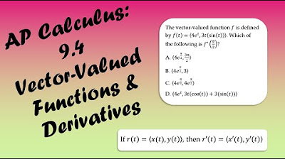
What is the instantaneous rate of change of a vector-valued function?
-The instantaneous rate of change of a vector-valued function is represented by its derivative, denoted as F(t) = <4t - 7t^2, 6 + 2t - t^2> in the given example, which provides the rate of change for each component of the vector function H(t).
How can you find the value of H(0) given the instantaneous rate of change F(t) and H(1)?
-To find H(0), you integrate the components of F(t) to find the function H(t), and then use the given H(1) = (2, 7) to solve for the constants of integration. By plugging in t=1, you can determine the values of C1 and C2, and then evaluate H(t) at t=0 to find H(0).
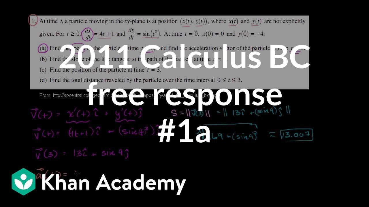
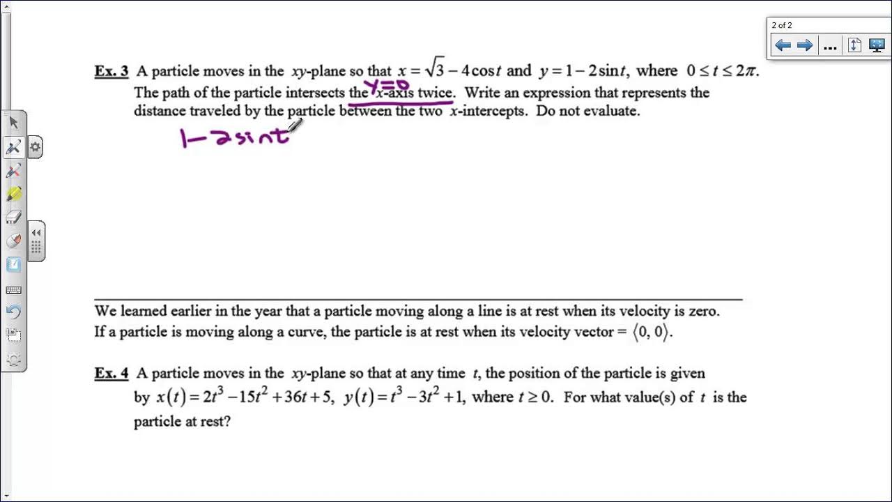
In the context of a particle moving along a curve, how can you find the position of the particle at a given time?
-To find the position of the particle at a given time, you use the velocity vector to determine the derivatives of the x and y coordinates (x'(t) and y'(t)), and then apply the fundamental theorem of calculus to integrate these derivatives from the initial time to the desired time, using the initial position as a starting point.
What is the x-coordinate of the particle at time T=3 given its velocity vector and initial position?
-The x-coordinate of the particle at time T=3 is found by integrating the x-component of the velocity vector from T=2 to T=3 and adding the initial x-coordinate. In this case, it is calculated as 2 (initial x-coordinate) + ∫ from 2 to 3 of sin(1.75t + 3) dt, which evaluates to 4.172.
What is the y-coordinate of the particle at time T=11 given its velocity vector and initial position?
-The y-coordinate of the particle at time T=11 is found by integrating the y-component of the velocity vector from T=2 to T=11 and adding the initial y-coordinate. It is calculated as -3 (initial y-coordinate) + ∫ from 2 to 11 of (ln(0.6t + 2))^3 dt, which evaluates to 47.792.
Outlines
📚 Introduction to Integrating Vector-Valued Functions
This paragraph introduces the concept of integrating vector-valued functions, building upon the previous lesson on differentiation. It explains that both indefinite and definite integration can be applied to vector-valued functions, which are functions with components X and Y depending on a parameter T. The process involves finding the antiderivatives of the components and combining them with constants to form the antiderivative of the entire vector function. An example is provided to illustrate the integration process, including the use of initial conditions to solve for these constants.
🧮 Example of Integrating a Vector-Valued Function
The paragraph walks through a specific example of integrating a given vector-valued function, G'(T), which has an initial condition G(0) = (1, 2). The function is integrated by separating its components and finding the antiderivative of each. The constants of integration are determined by applying the initial condition. The paragraph also introduces the concept of definite integration for vector-valued functions and provides another example, calculating the integral of a vector function f(T) from 0 to 2.
🌟 Finding Instantaneous Rate of Change for Vector Functions
This section discusses the application of integrating vector-valued functions to find the instantaneous rate of change, using the function h(t) as an example. It explains how to find the function H(t) by integrating its instantaneous rate of change, F(t). The process involves integrating both components of F(t) and using given initial conditions to solve for the constants of integration. The paragraph concludes with a multiple-choice question related to the topic, where the correct answer is derived by applying the integration concepts discussed.
🚀 Application: Particle Motion and Integration
The final paragraph applies the concepts of vector-valued function integration to a real-world scenario of a particle moving along a curve in the XY plane. The particle's position and velocity vectors are given, and the task is to find the particle's coordinates at specific times. The paragraph outlines the process of using the velocity vector to find the position by integrating the derivative of the position function over time intervals. It provides detailed steps and calculations to find the x and y coordinates of the particle at times T=3 and T=11, demonstrating the practical use of integration in motion analysis.
Mindmap
Keywords
💡Vector-valued functions
💡Integration
💡Antiderivatives
💡Constants of integration
💡Definite integration
💡Instantaneous rate of change
💡Position vector
💡Velocity vector
💡Initial conditions
💡Integration by parts
💡Kinematics
💡Accumulation
Highlights
The lesson focuses on integrating vector-valued functions, which is the opposite process of differentiation.
Vector-valued functions can be integrated both indefinitely and definitely, similar to scalar functions.
A vector-valued function is represented with components X and Y, with respect to a parameter T.
Integration of vector-valued functions involves taking the integral of each component separately.
The antiderivative of a vector-valued function is represented with the same components, with additional constants.
An example is provided to demonstrate the process of integrating a vector-valued function and finding the constants.
The initial condition is used to find the constants in the antiderivative of a vector-valued function.
Definite integration of vector-valued functions is performed by integrating each component within the given bounds.
A second example is given to illustrate the process of definite integration for a vector-valued function.
The instantaneous rate of change of a vector-valued function is given by its derivative, which can be represented as a vector.
To find the function at a specific time, the integral of the derivative is taken from an initial time to the desired time.
The position of a particle at a given time can be found by integrating its velocity vector from an initial position.
The x-coordinate of a particle's position at time T equals three is calculated using the velocity vector's x-component.
The y-coordinate of a particle's position at time T equals 11 is calculated using the velocity vector's y-component.
The use of a graphing calculator is suggested for evaluating integrals in the context of vector-valued functions.
The final x-coordinate of the particle at time T equals three is found to be 4.172.
The final y-coordinate of the particle at time T equals 11 is found to be 47.792.
Transcripts


5.0 / 5 (0 votes)
Thanks for rating: