Local linearization
TLDRThis video script delves into the concept of local linearization, a method to approximate complex functions with simpler linear ones. It starts by identifying a specific input point and then constructs a new function, L, that represents a tangent plane to the original function's graph at that point. The script explains the process of finding partial derivatives, evaluating them at the input point, and using them to formulate the linear approximation. It also introduces the gradient and dot product in the context of vector notation, showing how these concepts simplify the linearization process. The goal is to create a more compact and general expression that can be applied to functions with multiple variables, making it easier to approximate and compute.
Takeaways
- 📚 The script discusses the concept of local linearization, which is a method to approximate a function with a simpler, linear one at a specific point.
- 🔍 Local linearization is useful for approximating complex functions with constant partial derivatives, making them easier to work with in calculations or programming.
- 📍 The process begins by identifying a specific input point, denoted as ( x_0 ) and ( y_0 ), where the approximation will be made.
- 📈 The function to be approximated is denoted as ( f ), and the linear approximation is represented as ( L ) or ( L_f ).
- 📝 To perform local linearization, one must first find the partial derivatives of ( f ) with respect to ( x ) and ( y ) and evaluate them at the input point ( x_0, y_0 ).
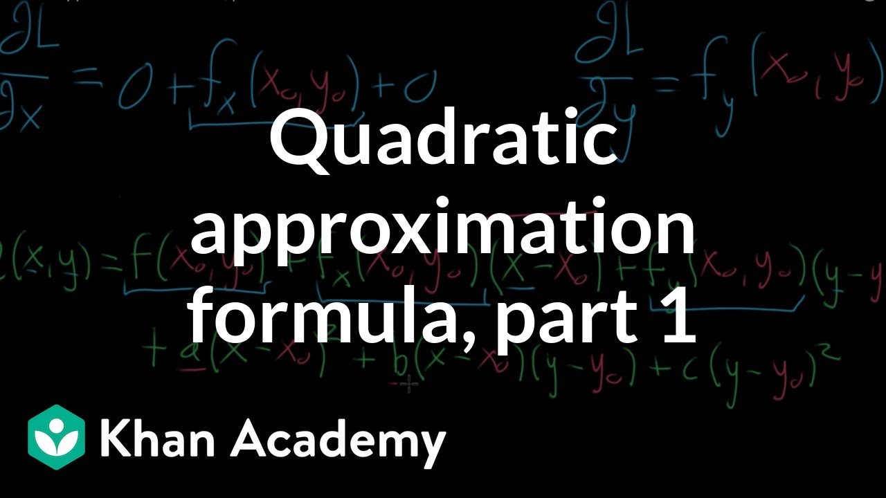
- 🔢 The linear approximation is constructed by multiplying the evaluated partial derivatives by the differences ( x - x_0 ) and ( y - y_0 ), respectively.
- ✅ The linear approximation function ensures that when evaluated at the input point itself, it equals the original function value at that point, due to the zeroing out of the variable terms.
- 📐 The term 'linear' in this context refers to the simplicity of the variable terms, which are each just multiplied by a constant, without any complex operations.
- 📚 The script introduces the concept of expressing the approximation in vector form, which is more compact, easier to remember, and applicable to functions with more than two variables.
- 📈 The gradient vector, evaluated at the input point, is used in the dot product to represent the linear part of the approximation.
- 📝 The final expression for local linearization combines the linear term, represented as a dot product, with the constant term, which is the function value at the input point.
Q & A
What is the main purpose of finding a tangent plane to a function's graph?
-The main purpose of finding a tangent plane to a function's graph is to approximate a potentially complicated function with a simpler one, specifically a linear function, which has constant partial derivatives and is easier to work with.
What is the term used to describe the process of approximating a function with a simpler one at a specific point?
-The process is called 'local linearization', which involves approximating the function near a specific input point with a linear function.
What are the steps to perform local linearization of a function with two inputs?
-The steps include finding the partial derivatives of the function with respect to each input variable, evaluating these derivatives at a specific input point, and then constructing a linear function that includes these derivatives multiplied by the differences from the input point, plus the original function value at that point.
Why is the process of local linearization useful even if the function is not linear in the technical sense?
-Local linearization is useful because it simplifies the function to a form where each variable is multiplied by a constant, making it easier to compute and approximate, even though the original function might not be technically linear.
How can the local linearization be represented in vector form?
-In vector form, local linearization can be represented using a dot product between the gradient vector (evaluated at the input point) and the difference between the variable vector and the input point vector, plus the function value at the input point.
What is the significance of the gradient in the context of local linearization?
-The gradient is significant because it contains the partial derivatives of the function with respect to each variable, which are essential components in constructing the linear approximation of the function.
Why is it important for the linearization to equal the function itself at the local point?
-It is important because the purpose of local linearization is to approximate the function near a specific point, and if the linearization equals the function at that point, it ensures the approximation is accurate at least at that point.
How does the local linearization method extend to functions with more than two input variables?
-The method extends by considering the input as a vector with multiple components, where each component corresponds to an input variable. The gradient is then a vector of partial derivatives, and the linearization process involves a dot product with the difference vector of the input variables.
What is the advantage of using vector notation in local linearization?
-Vector notation simplifies the process and makes it more general, allowing for easy application to functions with any number of input variables, not just two.
Can you provide an example of how local linearization might be used in practical applications?
-Local linearization can be used in practical applications such as machine learning algorithms for function approximation, in numerical methods for solving equations, or in economics for approximating demand functions near certain price points.
Outlines
📚 Introduction to Local Linearization
The script begins by revisiting the concept of local linearization, a method for approximating a complex function with a simpler linear one at a specific input point, denoted as x nought and y nought. The process involves finding the tangent plane to the graph of a function with two inputs. The local linearization is explained as a way to simplify the function with constant partial derivatives, making it easier to work with, especially in higher dimensions. The goal of the video is to express this concept in a more compact and general vector form, applicable to functions with more than two variables.
🔍 Vector Formulation of Local Linearization
This paragraph delves into the vector representation of the local linearization process. It starts by discussing the partial derivatives of the function with respect to x and y, evaluated at the input point x nought, y nought, and how these are used to form a linear approximation. The script introduces the concept of the gradient and explains how it can be used in conjunction with the difference between the variable vector x and the constant vector x nought to create a dot product. This dot product, along with the function's value at the input point, forms the linear approximation. The paragraph emphasizes the simplicity and generality of this vector approach, which can be extended to functions with any number of input variables, and concludes by highlighting the practical applications of this method in approximating functions for computational efficiency or when the exact function form is unknown.
Mindmap
Keywords
💡Tangent Plane
💡Local Linearization
💡Partial Derivative
💡Input Point
💡Function Approximation
💡Constant Partial Derivatives
💡Vector Form
💡Gradient
💡Dot Product
💡Linear Function
Highlights
Local linearization is a method to approximate a function with a simpler, linear function at a specific input point.
The linearization process involves finding the tangent plane to the graph of a function with two inputs.
A new function L, or L sub f, is created to represent the tangent plane.
Local linearization is useful for approximating complex functions with constant partial derivatives.
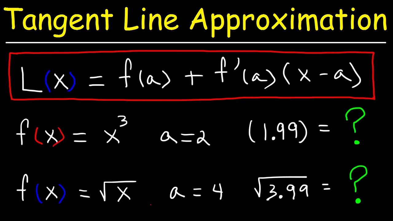
The linearization function L is constructed by evaluating the partial derivatives of the original function at the input point and multiplying by the difference from the input point.
The linear approximation ensures that it equals the original function at the specified input point.
The term 'linear' in this context refers to the variables being multiplied by constants without any complex operations.
Vector notation can be used to represent the input points and partial derivatives more compactly.
The gradient vector is used to represent the partial derivatives evaluated at the input point.
The linearization can be expressed as a dot product between the gradient vector and the difference vector from the input point.
The linear term in the linearization represents the variable components multiplied by constants.
The constant term in the linearization is the value of the original function evaluated at the input point.
The linearization expression simplifies to a function that is easier to compute than the original function.
Local linearization can be applied to functions with more than two input variables by using vector notation.
The method provides an approximation of the function and its gradient near a specified point.
An article is available for further examples and applications of local linearization.
Transcripts
Browse More Related Video


5.0 / 5 (0 votes)
Thanks for rating: