Calculus 3: Motion in Space: Velocity and Acceleration (Video #10) | Math with Professor V
TLDRThis calculus video lecture delves into the concepts of motion, space velocity, and acceleration. It explains how to derive velocity and acceleration from a position vector function, using the given example of R(t) = rad(t) and 1 - t. The lecture also covers the calculation of speed, sketching the path, velocity, and acceleration vectors, and introduces tangential and normal components of acceleration. It further explores the relationship between normal component of acceleration, curvature, and speed squared, providing an intuitive understanding and examples to solidify these advanced calculus topics.
Takeaways
- 📚 The lecture introduces the concepts of motion in space, focusing on velocity and acceleration as they relate to calculus three.
- 🚀 R(t) is defined as the position vector, indicating the location of a particle at time t, with its derivative R'(t) representing velocity, V(t).
- 🔍 Velocity is a vector that is tangent to the curve, and its magnitude represents speed, denoted as |V(t)| or ds/dt.
- 🔄 The second derivative R''(t), or V'(t), represents acceleration, A(t), which is the rate of change of velocity with respect to time.
- 📈 The script provides a step-by-step example of finding the velocity, acceleration, and speed of a particle given the position function R(t) = √(t) and 1 - t.
- 📊 The importance of sketching the path of a particle, along with velocity and acceleration vectors at specific points, is emphasized for visual understanding.
- 🧭 The process of eliminating the parameter to identify the curve in the XY plane is discussed as a method for graphing the particle's path.
- 🔬 Anti-differentiation is used to find velocity vectors from given acceleration vectors and initial conditions, leading to the position vector.
- 📐 The script explains how to represent acceleration in terms of its tangential and normal components, which are useful for understanding motion.
- 🌐 Curvature is introduced as a concept related to the normal component of acceleration, with a formula provided for its calculation.
- 🔑 The video concludes with an application of the concepts to prove Kepler's first law of motion, showing the practical use of these mathematical tools in astronomy.
Q & A
What is the position vector R(t) in the context of this calculus lecture?
-The position vector R(t) represents the location of a particle at time 't' in a given motion problem.
What does the derivative of R(t), also known as R'(t), indicate?
-R'(t), or the derivative of R(t), provides the rate of change in position with respect to time, which is also known as velocity, represented as V(t).
How is the velocity vector related to the curve traced by the particle's motion?
-The velocity vector is tangent to the curve at any given point, and its magnitude represents the speed of the particle.
What is the second derivative of R(t), and what does it represent?
-The second derivative of R(t), denoted as R''(t) or V'(t), represents the rate of change in velocity with respect to time, which is known as acceleration, represented as a(t).
How can you find the velocity and acceleration of a particle given its position function R(t) = sqrt(t) and 1 - t?
-To find the velocity, you differentiate R(t) with respect to t to get V(t). To find the acceleration, you differentiate V(t) with respect to t to get a(t).
What is the magnitude of the velocity vector V(t) when t = 1 for the given position function?
-The magnitude of V(t) when t = 1 is the square root of the sum of the squares of the components of V(1), which in this case is sqrt((1/2)^2 + (-1)^2) = sqrt(1/4 + 1) = sqrt(5/4).
How can you sketch the path of a particle given its position function?
-You can sketch the path by eliminating the parameter 't' and identifying the curve in the XY plane, or by making a table of values for 't' and plotting the corresponding 'x' and 'y' coordinates.
What are the components of the acceleration vector a(t) when t = 1 for the given position function?
-The components of the acceleration vector a(1) are found by differentiating the velocity vector V(t) and evaluating at t = 1, which yields (-1/4, 0).
How can you find the position vector R(t) given an acceleration vector and initial conditions?
-You anti-differentiate the acceleration vector twice, applying the initial conditions for velocity and position at the starting time to solve for constants of integration.
What is the difference between the tangential and normal components of acceleration?
-The tangential component of acceleration (a_t) is the component along the direction of motion, while the normal component of acceleration (a_n) is perpendicular to the direction of motion.
How is the curvature of a curve related to the normal component of acceleration?
-Curvature is equal to the normal component of acceleration divided by the magnitude of the velocity vector squared, or equivalently, the magnitude of the position vector's derivative cubed.
Outlines
📚 Introduction to Motion and Space: Calculus in Vector Functions
This paragraph introduces the concepts of motion in space using calculus with vector functions. The position vector R(t) represents the location of a particle at time t, with its first derivative, R'(t), giving the velocity vector, which is tangential to the particle's path. The magnitude of the velocity vector, |V(t)|, represents the speed of the particle. The second derivative, R''(t), is the acceleration vector, which describes how the velocity changes over time. The paragraph sets the stage for finding the velocity, acceleration, and speed of a particle given its position function R(t) = (r(t), 1 - t), and includes a sketch of the particle's path and the vectors at t = 1.
🔍 Deriving Velocity and Acceleration Vectors from Position Function
The paragraph focuses on deriving the velocity and acceleration vectors from a given position function. It explains the process of taking the first and second derivatives of the position vector to obtain the velocity vector V(t) and acceleration vector A(t), respectively. The example provided uses the position function R(t) = (r(t), 1 - t), resulting in velocity and acceleration vectors at t = 1. The paragraph also discusses the concept of speed, which is the magnitude of the velocity vector, and includes a calculation for the speed of the particle at t = 1.
📈 Sketching the Path and Vectors for a Particle's Motion
This paragraph delves into the process of sketching the path of a particle and its associated velocity and acceleration vectors. It suggests methods such as creating a table or eliminating the parameter to identify the curve in the XY plane. The example provided involves writing parametric equations for x and y, and then graphing a parabola that opens downward and is shifted up one unit. The paragraph also discusses the inclusion of velocity and acceleration vectors at a specific point (1,0) on the graph.
🔄 Anti-Differentiation to Find Position Vectors from Acceleration
The paragraph discusses the process of anti-differentiating acceleration vectors to find velocity and position vectors, given initial conditions. It provides a step-by-step method to anti-differentiate the acceleration vector to obtain the velocity vector, and then to find the position vector R(t). The example includes solving for constants using initial conditions and the final expression for the position vector as polynomials in t.
🧭 Decomposing Acceleration into Tangential and Normal Components
This paragraph explains the decomposition of the acceleration vector into its tangential and normal components with respect to the motion of a particle along a curve. It introduces the concept of the unit tangent vector and the normal vector, and how to calculate the tangential component of acceleration using the scalar projection of the acceleration vector along the unit tangent. The paragraph also covers the calculation of the normal component of acceleration and its relationship with curvature.
🌌 Applying Formulas for Acceleration Components and Curvature
The paragraph demonstrates the application of formulas for calculating the tangential and normal components of acceleration and curvature at a specific point in time. It provides an example using a position function R(t) with exponential terms, showing the process of taking derivatives and applying the formulas to find the components of acceleration and curvature at t = 0. The paragraph also generalizes the process for any time t, leaving the values in terms of t.
🚀 Conclusion and Kepler's First Law of Motion
In the concluding paragraph, the lecture notes are summarized, and an invitation is extended to explore the proof of Kepler's first law of motion using the concepts covered in the chapter. The paragraph highlights the relevance of the material to understanding planetary motion around the Sun in elliptical orbits, with the Sun at one focus.
Mindmap
Keywords
💡Position Vector
💡Velocity
💡Acceleration
💡Speed
💡Tangential Component of Acceleration
💡Normal Component of Acceleration
💡Curvature
💡Parametric Equations
💡Scalar Projection
💡Anti-differentiation
Highlights
Introduction to calculus three concepts of motion, space velocity, and acceleration.
Explanation of position vector R(t), velocity vector V(t), and acceleration vector A(t).
Velocity vector's tangential relationship to the curve and its magnitude as speed.
Derivation of velocity and acceleration from a given position function R(t) = r(t) and 1 - t.
Finding the velocity vector V(1) at a specific point on the curve.
Calculation of acceleration vector A(1) at the same point.
Determination of speed as the magnitude of velocity at time T.
Sketching the path of a particle in the XY plane using parametric equations.
Graphical representation of velocity and acceleration vectors at a given point.
Anti-differentiation to find velocity and position vectors from acceleration.
Use of initial conditions to solve for constants in velocity and position vectors.
Differentiating between the components of acceleration: tangential and normal.
Intuitive explanation of tangential and normal components of acceleration.
Calculation of the tangential component of acceleration using scalar projection.
Derivation of the normal component of acceleration and its relation to curvature.
Application of the formulas for tangential and normal components of acceleration in an example.
Demonstration of the relationship between normal component of acceleration, curvature, and speed.
Proof of Kepler's first law of motion using concepts from the chapter.
Transcripts
Browse More Related Video
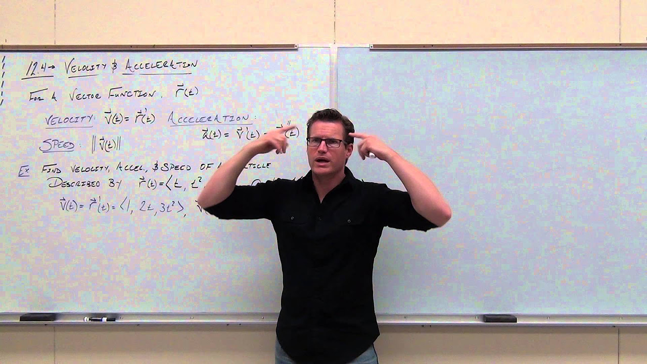
Calculus 3 Lecture 12.4: Velocity and Acceleration of Vector Functions
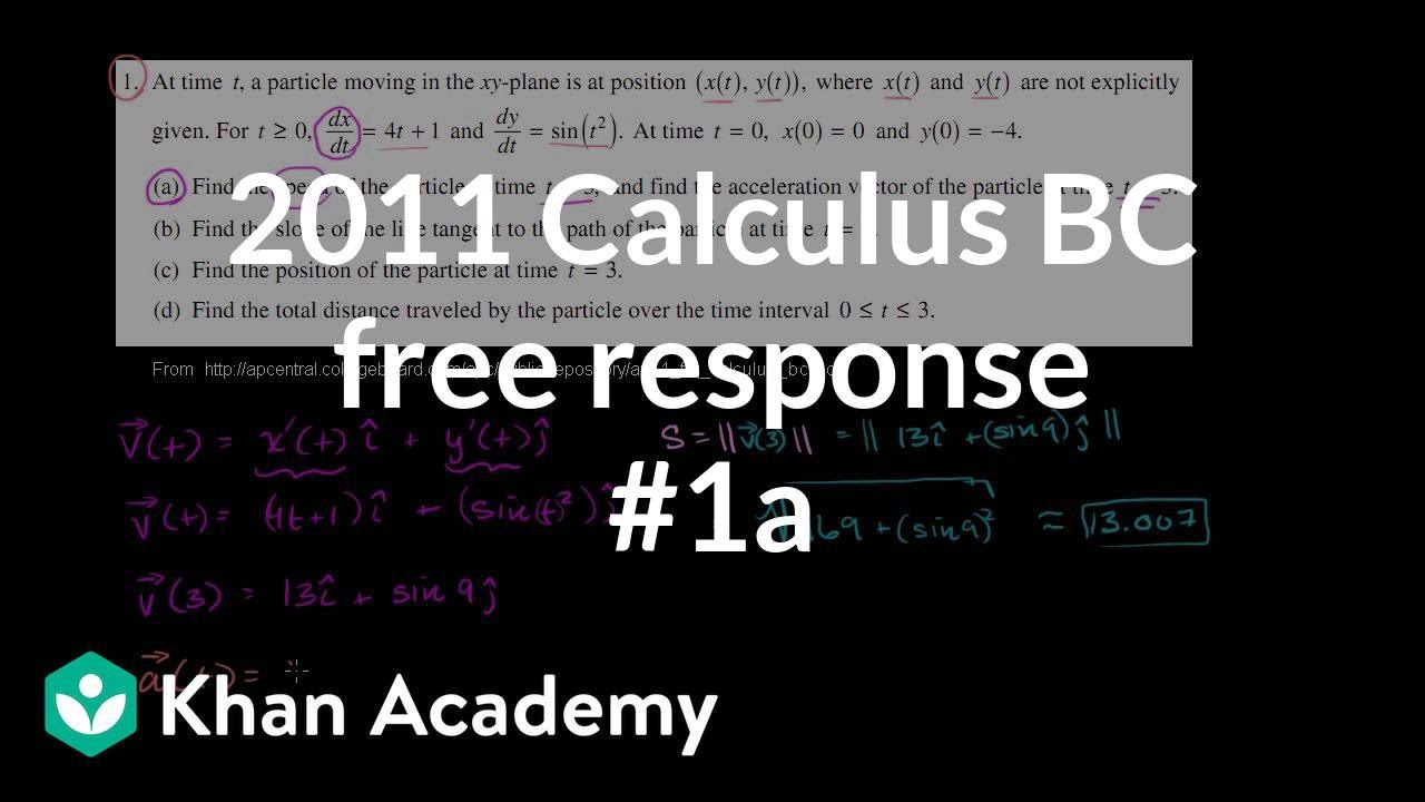
2011 Calculus BC free response #1a | AP Calculus BC solved exams | AP Calculus BC | Khan Academy
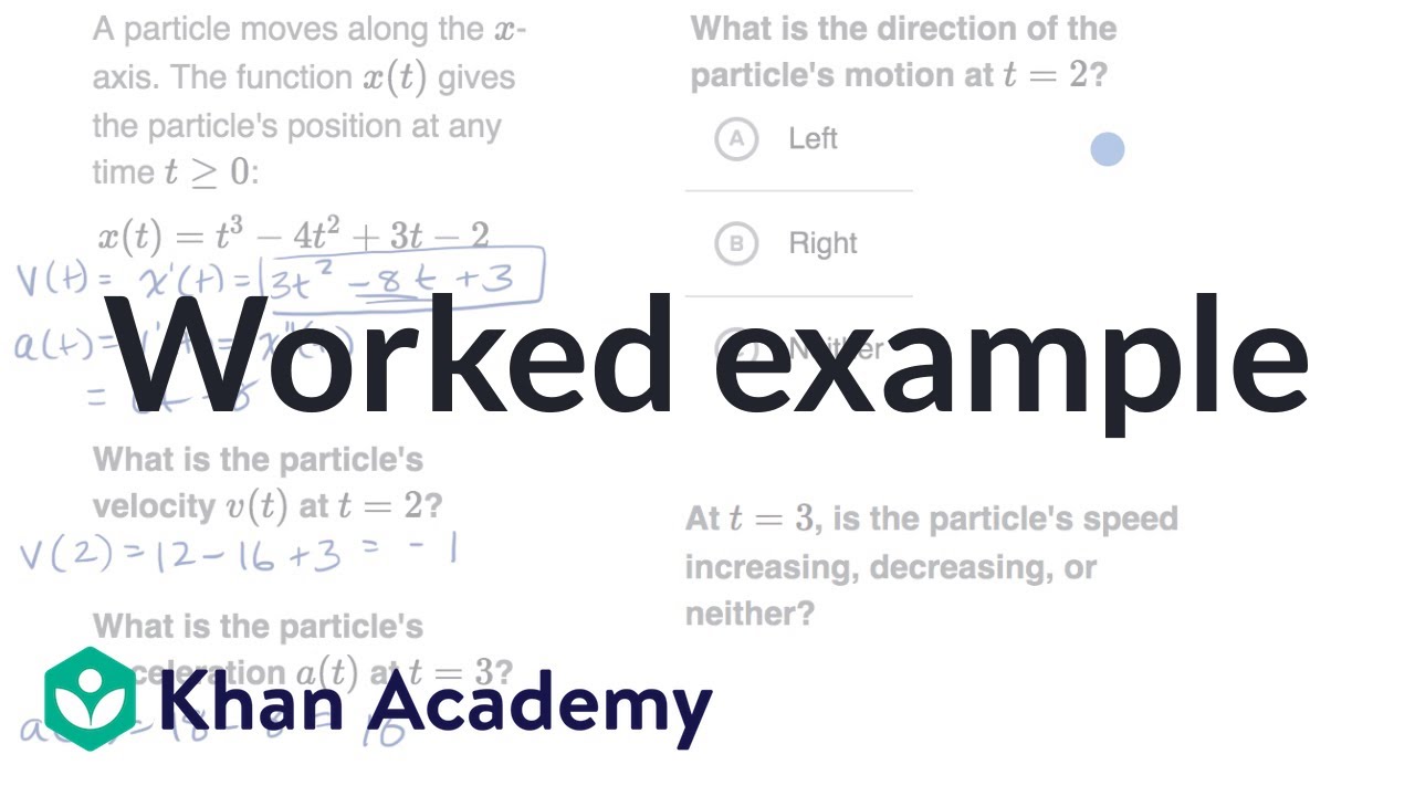
Worked example: Motion problems with derivatives | AP Calculus AB | Khan Academy
College Physics 1: Lecture 8 - Acceleration

8.01x - Lect 2 - 1D Kinematics - Speed, Velocity, Acceleration
Calculus - Position Average Velocity Acceleration - Distance & Displacement - Derivatives & Limits
5.0 / 5 (0 votes)
Thanks for rating: