Elementary Stats Lesson #14

walter dorman

7 Mar 202138:38

EducationalLearning

32 Likes 10 Comments

TLDRThe lecture delves into the concept of sampling distributions, focusing on the sample proportion from chapter eight of the textbook. It revisits the sample mean, then explores the sample proportion's notation, behavior, and distribution. The instructor uses real-world examples to illustrate calculating proportions and emphasizes the importance of sample size in controlling variability. The central limit theorem is discussed for both sample means and proportions, highlighting conditions for their normal distribution. The lecture concludes with applications of these concepts to answer probability questions related to sample proportions.

Takeaways

📚 The lesson focuses on understanding the sampling distribution for the sample proportion, which is the second half of chapter eight in the textbook.
🔍 The sample proportion (p-hat) is used to estimate the population proportion and is calculated by dividing the number of successes in a sample by the sample size.
🌟 The mean of the sampling distribution for the sample proportion is equal to the true population proportion (p).
📉 The standard error of the sample proportion is calculated as the square root of the product of the population proportion (p), the failure rate (1-p), and the inverse of the sample size (n).
📈 The central limit theorem applies to sample proportions, stating that the distribution of p-hat is approximately normal if the sample size is large enough.
✅ The condition for the normal approximation of p-hat is that the product of the sample size (n), the population proportion (p), and 1-p is at least 10.
🤔 The script discusses the potential for variability in sample proportions, emphasizing that different samples may yield different p-hat values.
📝 The transcript includes examples of calculating sample proportions, such as the proportion of individuals who wear contacts or like having classes on Fridays.
🧐 The lesson explores the use of p-hat as an estimator for the population proportion and the importance of sample size in refining this estimation.
📉 The transcript explains the concept of standard error and its role in understanding the variability of the sample proportion distribution.
🔢 The script provides a step-by-step guide on how to check for normality, compute the mean and standard deviation of p-hat, and use these to answer probability questions related to sample proportions.

Q & A

What is the main topic of chapter eight in the textbook?
-The main topic of chapter eight is sampling distributions, specifically focusing on the sampling distribution for the sample proportion.
What is the notation for the sample mean and what does it represent?
-The notation for the sample mean is \( \bar{x} \), which represents the mean from a simple random sample of size \( n \) drawn from a population.
What is the standard deviation of the sampling distribution of the sample mean, and what is it commonly referred to as?
-The standard deviation of the sampling distribution of the sample mean is denoted as \( \sigma_{\bar{x}} \), and it is commonly referred to as the standard error of the mean.
Under what conditions does the sample mean have an approximately normal distribution according to the central limit theorem?
-The sample mean has an approximately normal distribution if the population is approximately normal or if the sample size is large enough, typically 30 or larger.
What is the notation used to represent the sample proportion and what does it signify?
-The notation for the sample proportion is \( \hat{p} \), which signifies the proportion of successes in a simple random sample.
What is the mean of the sampling distribution for the sample proportion?
-The mean of the sampling distribution for the sample proportion, denoted as \( \mu_{\hat{p}} \), is equal to the true population proportion \( p \).
How is the standard error of the sample proportion calculated?
-The standard error of the sample proportion is calculated as the square root of the true population proportion \( p \) times the true failure rate \( 1 - p \), divided by the sample size \( n \).
What condition must be met for the sample proportion to have an approximately normal distribution?
-The sample proportion \( \hat{p} \) will have an approximately normal distribution if the sample size is large enough such that \( n \times p \times (1 - p) \) is greater than or equal to 10.
What is the significance of the sample proportion in statistical inference?
-The sample proportion is used as an estimate for the population proportion and is the basis for making inferences about the population from sample data.
What happens if the check for normality of the sample proportion fails, i.e., \( n \times p \times (1 - p) < 10 \)?
-If the check for normality fails, we cannot assume that the sample proportion has an approximately normal distribution. Instead, we must use the binomial distribution to compute probabilities of certain outcomes.

Outlines

00:00

📚 Introduction to Sampling Distributions for Sample Proportion

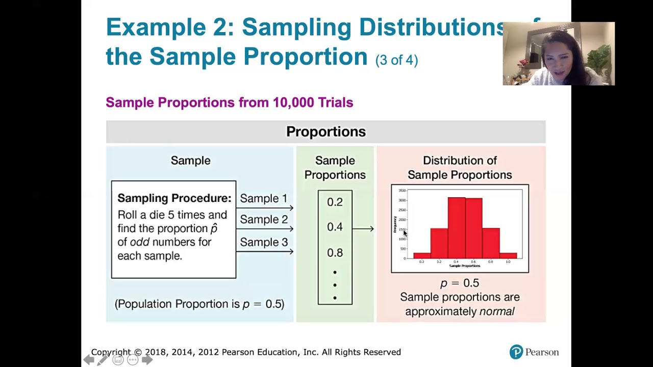
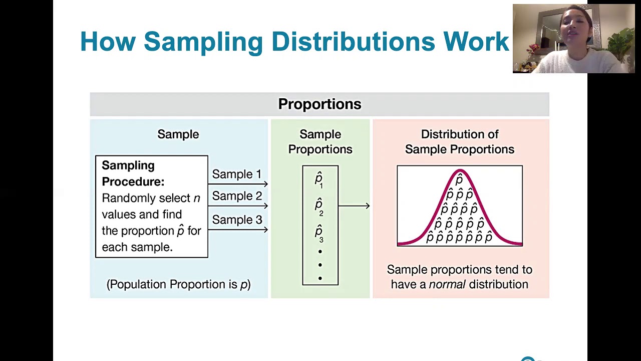
The lesson begins with an introduction to chapter eight of the textbook, focusing on sampling distributions, specifically the sampling distribution for the sample proportion. The instructor reviews the concept of the sample mean from the previous lesson, including its notation and standard deviation. The central limit theorem is discussed, highlighting the conditions under which the sample mean has an approximately normal distribution. The lesson then shifts to the sample proportion, explaining its relevance and how it differs from the sample mean, especially in scenarios involving binary outcomes like yes/no characteristics.

05:02

🔍 Understanding Sample Proportion and Its Distribution

The instructor delves deeper into the sample proportion, discussing its notation and how it is used in scenarios with binary outcomes. Two examples are provided to illustrate the calculation of the sample proportion. The importance of the sample proportion as an estimator for the population proportion is emphasized, and the concept of a crude estimate is introduced. The lesson also explores the variability of the sample proportion and introduces the standard error of the sample proportion, explaining how it can be controlled through sample size.

10:03

📉 Central Limit Theorem for Sample Proportion

This section discusses the central limit theorem as it applies to the sample proportion, explaining the conditions necessary for the sample proportion to have an approximately normal distribution. The instructor provides a formula for calculating the standard error of the sample proportion and explains how the sample size affects its variability. The importance of ensuring a large enough sample is stressed, with a specific condition involving the product of the sample size, population proportion, and the complement of the population proportion.

15:06

🤔 Analyzing Sample Proportion with Real-World Data

The instructor applies the concepts learned to real-world data, using examples from the National Center for Health Statistics and a survey about opinions on Friday classes. The process of checking sample size for normality, calculating the mean and standard error of the sample proportion, and using these values to answer probability questions is demonstrated. The calculations show how to determine the likelihood of observing certain sample proportions, given the population proportion.

20:08

📝 Describing the Sampling Distribution of Sample Proportion

The lesson continues with a detailed explanation of how to describe the sampling distribution of the sample proportion. The steps include checking for normality, computing the mean and standard error, and using these parameters to answer probability questions. The instructor uses various scenarios to illustrate these steps, including a study about hearing trouble among Americans and another about college students using headphones.

25:09

📉 Sample Proportion in Context of Pew Research Center Data

The instructor uses data from the Pew Research Center to describe the sampling distribution of the sample proportion regarding the belief that marriage is obsolete. The process of checking for normality, calculating the mean and standard error, and answering probability questions is demonstrated. The lesson shows how to determine the likelihood of observing certain sample proportions in a large sample of adult Americans.

30:09

🚫 Handling Small Sample Sizes in Sample Proportion Analysis

The final part of the lesson addresses what happens when the sample size is not large enough for the sample proportion to be considered approximately normal. The instructor explains that when the check for normality fails, one must revert to using binomial distribution calculations to determine probabilities. This section provides an alternative method for analyzing sample proportions when the conditions for a normal distribution are not met.

Mindmap

Keywords

💡Sampling Distribution

A sampling distribution is the probability distribution of a given statistic based on a random sample. In the video, the concept is central as it discusses how the distribution of the sample proportion and sample mean behave when samples are taken from a population. The script explains that the mean of the sampling distribution of the sample mean (x̄) is equal to the population mean (μ), and the standard deviation of this distribution, known as the standard error, is the population standard deviation (σ) divided by the square root of the sample size (n).

💡Sample Proportion

The sample proportion, denoted as p̂ (p-hat), is the ratio of the number of successes in a sample to the sample size, used to estimate the population proportion. The video script uses the sample proportion to discuss its distribution properties, such as its mean and standard error, and how it can be used to make inferences about the population from sample data.

💡Standard Error

The standard error is a measure that helps to understand the accuracy of the sample mean or proportion as an estimate of the population mean or proportion. In the script, the standard error of the mean (x̄) is calculated as the population standard deviation (σ) divided by the square root of the sample size (n). Similarly, the standard error of the sample proportion (p̂) is the square root of the product of the population proportion (p), its complement (1-p), and the sample size (n) inverse.

💡Central Limit Theorem

The Central Limit Theorem (CLT) is a statistical theory that states that the distribution of sample means (or sums) approaches a normal distribution as the sample size gets larger, regardless of the population's distribution shape. The video script refers to the CLT in the context of both the sample mean and the sample proportion, explaining that for sufficiently large sample sizes, the sampling distribution of these statistics will be approximately normal.

💡Population Proportion

The population proportion is the ratio of the number of individuals in a population with a specific characteristic to the total number of individuals in the population. In the video, the script uses the population proportion (p) to discuss how the sample proportion (p̂) is used to estimate it and how the variability of p̂ is related to the population proportion.

💡Normal Distribution

A normal distribution, also known as a Gaussian distribution, is a probability distribution that is characterized by its symmetry and the presence of a mean and standard deviation. The video script discusses the conditions under which the sampling distribution of the sample mean and sample proportion can be approximated as normal, which is important for making statistical inferences.

💡Sample Size

Sample size refers to the number of individuals in the sample. The script emphasizes the importance of sample size in determining the accuracy of the sample mean and proportion as estimates of the population parameters. A larger sample size reduces the standard error, leading to a more precise estimate.

💡Statistical Inference

Statistical inference is the process of drawing conclusions about a population from sample data. The video script foreshadows the use of sample proportions for statistical inference, indicating that the knowledge acquired about the behavior of sample proportions will be used to make inferences about population proportions.

💡Binomial Setting

The binomial setting refers to scenarios where there are exactly two mutually exclusive outcomes of a trial, often categorized as 'success' and 'failure'. The script mentions that if the sample size is not large enough for the Central Limit Theorem to apply, probabilities can still be calculated using binomial distribution methods, such as binomcdf, which calculates the cumulative probability of obtaining a certain number of successes or fewer.

💡Normalcdf Function

The normalcdf function is a statistical tool used to calculate the cumulative probability of a normal distribution up to a certain value. In the script, the function is used to determine the probability that the sample proportion (p̂) falls within a certain range, which is key for making inferences about the population proportion.

Highlights

Introduction to Chapter 8 material focusing on sampling distributions, specifically the sampling distribution for the sample proportion.

Review of the sample mean (x-bar) and its properties, including mean and standard deviation of the sampling distribution.

Explanation of the standard error of the mean and its relationship with sample size.

Introduction of the sample proportion (p-hat) and its relevance in scenarios involving binary outcomes.

Examples of calculating the sample proportion, such as the proportion of individuals wearing contacts or liking Friday classes.

The importance of the sample proportion as an estimator for the population proportion.

Understanding the variability of p-hat and its standard error in relation to the sample size.

The central limit theorem's application to the sample proportion and the conditions for its approximation to a normal distribution.

Calculation of probabilities involving the sample proportion using the normal distribution, given a large enough sample size.

Analysis of the probability that at most 12% of a sample have hearing trouble, with a real-world application to American demographics.

Interpretation of sample proportions in the context of headphone use and hearing trouble, suggesting potential associations.

Steps for analyzing the sampling distribution of p-hat, including checking for normality and computing mean and standard deviation.

Application of sample proportion knowledge to a scenario involving college students and text messaging habits.

Description of the sampling distribution of p-hat in a scenario with a large population and a sample size of 500, with a true population proportion of 0.4.

Calculation of probabilities for different events, such as less than 38% or between 40% and 45% believing marriage is obsolete.

Discussion on what happens when the sample size is not large enough for the central limit theorem to apply, and the use of binomial calculations as an alternative.

Conclusion and transition to the next lesson, which will cover statistical inference procedures using the knowledge acquired about sample proportions.

Transcripts

Browse More Related Video

Elementary Stats Lesson #13

6.3.2 Sampling Distributions and Estimators - Sampling Distribution of Sample Proportions

WHAT IS A "SAMPLING DISTRIBUTION" and how is it different from a "sample distribution"... and stuff

Top 10 Tips for AP Statistics Unit 5 Sampling Distributions

Sampling distribution of the sample mean 2 | Probability and Statistics | Khan Academy

6.3.1 Sampling Distributions and Estimators - Sampling Distributions Described and Defined

Related Tags

Sampling Distribution Statistics Lesson Sample Proportion Central Limit Theorem Normal Distribution Standard Error Population Proportion Statistical Inference Data Analysis Research Methodology