Elementary Stats Lesson #3 B
TLDRThis educational video script explains the concept of standard deviation as a measure of data spread, both for a population (σ) and a sample (s). It clarifies the process of calculating these values and emphasizes the importance of using the correct formula for each. The script also introduces the empirical rule, or 68-95-99.7 rule, which describes the distribution of data points around the mean in a symmetric, bell-shaped distribution. An example using the heights of men at a baseball game illustrates how to apply the rule to estimate various segments of a population.
Takeaways
- 📊 The script discusses the calculation of the population standard deviation (σ), which is the square root of the population variance, and its importance in understanding the spread of data.
- 📈 The standard deviation's square root also converts the units back to the original measurement scale, which helps in interpreting the spread in the context of the data.
- 🔢 A larger standard deviation indicates a more spread out dataset, while a smaller standard deviation suggests data points are closer to the mean.
- 🔧 When dealing with sample data instead of a population, the sample variance (s²) is calculated differently, using the formula that involves dividing by the degrees of freedom (n-1).
- 📐 The degrees of freedom, represented as n-1, is a concept that will frequently appear in statistical calculations, especially with sample data.
- 📉 The sample standard deviation (s) is the square root of the sample variance and provides an indication of how spread out the data points in a sample are from the sample mean.
- 🛠 Calculators can simplify the process of calculating variance or standard deviation, which is time-consuming when done by hand.
- 📊 The script mentions that the one-variable stats package in calculators can compute both population and sample standard deviations, as it cannot discern the nature of the data input.
- ⚠️ Both variance and standard deviation are not resistant to outliers or skewness in the data, which means they can be significantly affected by these factors.
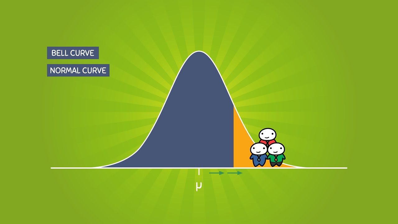
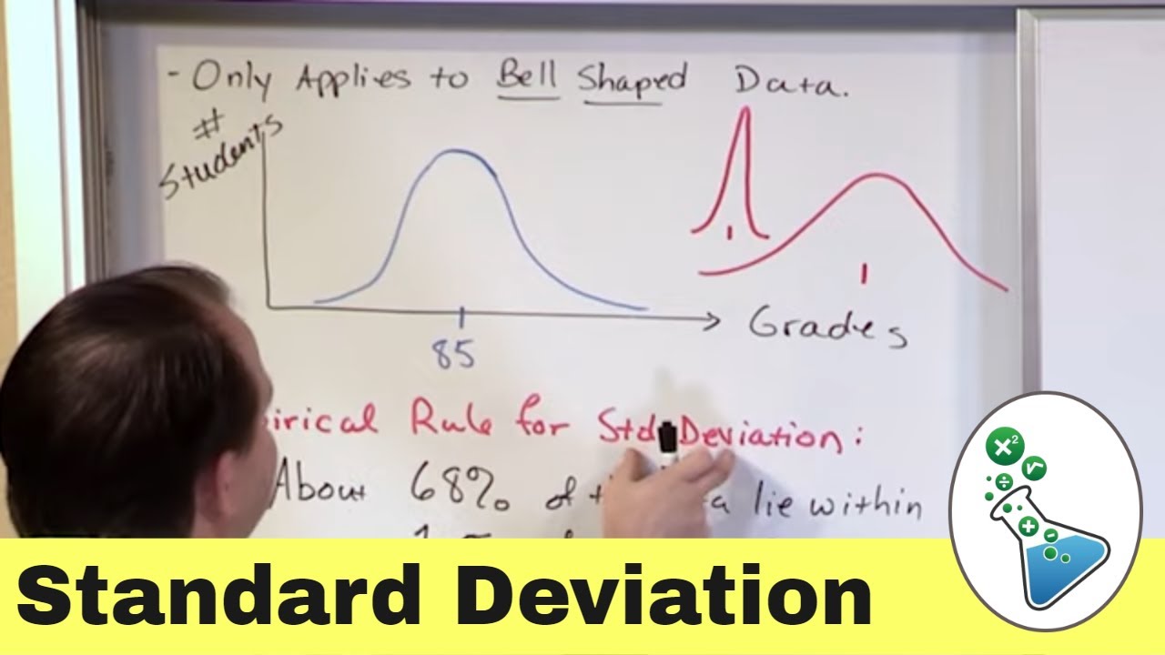
- 📘 The script introduces the empirical rule, also known as the 68-95-99.7 rule, which describes the distribution of data points in a symmetric, bell-shaped distribution relative to the mean and standard deviation.
- 📚 The empirical rule is a significant concept that connects descriptive statistics to further analysis, providing a framework for understanding data distribution and making inferences about the population.
Q & A
What is the standard deviation and how is it calculated?
-The standard deviation is a measure of the amount of variation or dispersion in a set of values. For a population, it is calculated as the square root of the population variance. If the data is from a sample, the sample standard deviation is the square root of the sample variance, which is the sum of the squared deviations from the mean divided by the sample size minus one (n-1).
Why is the square root taken when calculating standard deviation?
-The square root is taken to revert the squaring process used in calculating variance and to return to the original units of measurement. This also helps in interpreting the standard deviation as the average distance from the mean.
What does a larger standard deviation indicate about a data set?
-A larger standard deviation indicates that the data points are more spread out from the mean, suggesting greater variability in the dataset.
What is the difference between population variance and sample variance?
-Population variance is calculated using the entire population data, dividing the sum of squared deviations by the population size. Sample variance, on the other hand, is calculated from a subset of the population and divides the sum of squared deviations by the sample size minus one (n-1), which accounts for the sample being a part of the whole population.
What is the term used for sample size minus one and why is it significant?
-Sample size minus one is called 'degrees of freedom'. It is significant because it is used in statistical calculations to account for the number of independent pieces of information that can be obtained from the sample.
Why might the sample standard deviation be larger than the population standard deviation?
-The sample standard deviation might be larger due to the use of n-1 (degrees of freedom) in the denominator during calculation, which can result in a larger variance estimate for samples than for the entire population.
How can a calculator assist in calculating variance and standard deviation?
-Calculators, particularly those with a one-variable statistics package, can automate the process of calculating variance and standard deviation, making it less time-consuming and reducing the chance of manual errors.
What is the empirical rule, and how does it relate to the standard deviation and mean?
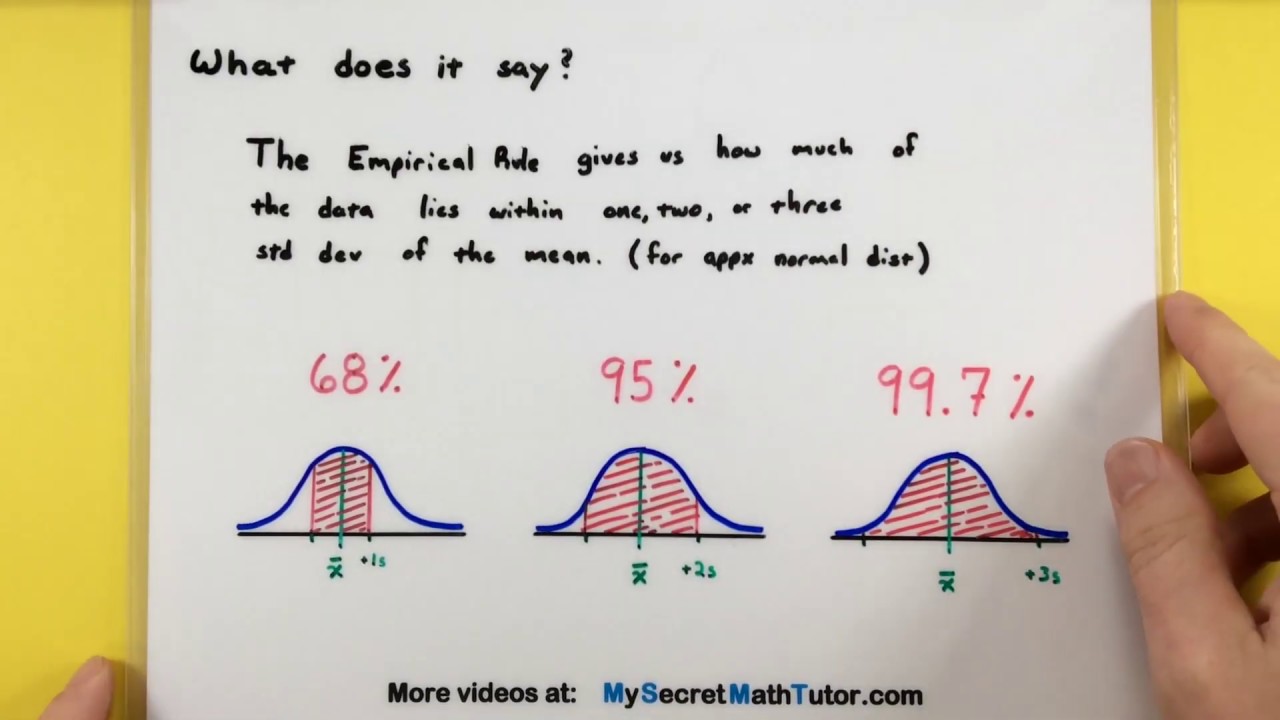
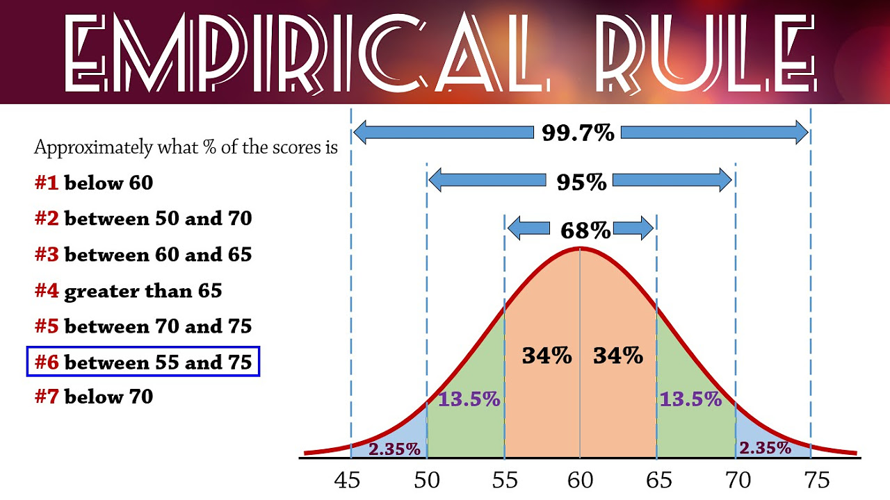
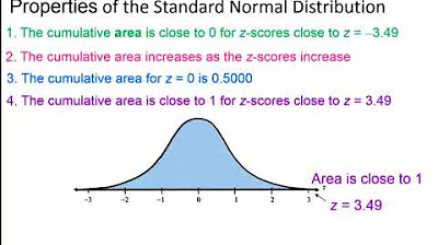
-The empirical rule, also known as the 68-95-99.7 rule, describes the distribution of data points around the mean in a normal (bell-shaped) distribution. It states that approximately 68% of the data falls within one standard deviation of the mean, 95% within two standard deviations, and 99.7% within three standard deviations.
Why are the mean and standard deviation considered a numerical summary package for a dataset?
-The mean and standard deviation together provide a comprehensive summary of a dataset, especially for symmetric, bell-shaped distributions. They describe the central tendency and dispersion of the data, allowing for a quick understanding of the dataset's characteristics.
How can the empirical rule be applied to estimate the percentage of a population within certain height ranges?
-Using the empirical rule, one can estimate that approximately 68% of individuals fall within one standard deviation of the mean height, 95% within two standard deviations, and 99.7% within three standard deviations. This can be used to estimate the percentage of a population within specific ranges, given the mean and standard deviation of the heights.
What insights can be gained from the example of men's heights at a baseball game?
-The example illustrates how the empirical rule can be used to estimate the percentage of men within certain height ranges at a baseball game, given the mean and standard deviation of their heights. It also shows how to estimate the maximum and minimum heights and the number of men in specific height categories.
Outlines
📚 Understanding Standard Deviation and Variance
This paragraph explains the concept of standard deviation, both for a population and a sample. It begins with an apology for a technical error and then delves into calculating the standard deviation by taking the square root of the variance. The population variance for ladies' heights was given as 11.3 square inches, leading to a standard deviation of 3.4 inches. The importance of standard deviation in understanding data spread is emphasized, with a larger deviation indicating a more spread-out data set. The paragraph also discusses the difference between population and sample calculations, introducing the concept of 'degrees of freedom' and its relevance in sample data analysis. The use of a calculator for these calculations is suggested for efficiency, and the paragraph concludes with a note on the non-resistance of variance and standard deviation to outliers.
📉 The Empirical Rule and Data Distribution
This section introduces the empirical rule, also known as the 68-95-99.7 rule, which is a set of statistical measures that describe the distribution of data points in relation to the mean and standard deviation. It explains that for a symmetric, bell-shaped distribution, the mean and standard deviation provide a comprehensive summary of the data. The rule states that approximately 68% of data points fall within one standard deviation of the mean, 95% within two standard deviations, and 99.7% within three standard deviations. The paragraph uses the example of men's heights at a baseball game to illustrate how the empirical rule can be applied to estimate data segments and answer related questions, emphasizing the rule's significance in statistical analysis.
📏 Applying the Empirical Rule to Data Analysis
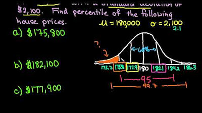
Building on the empirical rule, this paragraph provides a practical application by using the heights of men at a baseball game as an example. It describes how to visualize the data distribution as a bell-shaped curve and how to apply the empirical rule to estimate the percentage of individuals within certain height ranges. The mean height is given as 70 inches with a standard deviation of 2.5 inches. The paragraph calculates the percentage of men within one, two, and three standard deviations from the mean, providing specific numbers for each segment. It also addresses several hypothetical questions about the data set, such as the percentage of men taller than a certain height or estimating the height of the tallest man, demonstrating the empirical rule's utility in data analysis.
🤔 Analyzing Data Segments with the Empirical Rule
This paragraph continues the discussion on analyzing a data set using the empirical rule, focusing on how to answer specific questions about data segments. It provides a step-by-step breakdown of how to calculate the percentage of individuals within certain height ranges and estimates the number of men within those ranges using the given population size. The paragraph also addresses how to estimate the height of the tallest and shortest men at the game, using the empirical rule as a guide. It concludes with a note on the potential for further questions about various data segments, highlighting the empirical rule's importance in descriptive statistics.
👋 Closing Remarks and Looking Forward to Future Lessons
In the final paragraph, the speaker wraps up the lesson with well-wishes for the audience's safety and a successful semester. They encourage practice with the concepts learned through assignments on mymathlab and express anticipation for continuing the discussion on descriptive statistics in the next lesson. This closing paragraph serves as a transition, summarizing the importance of the topics covered and setting the stage for further exploration in subsequent lessons.
Mindmap
Keywords
💡Standard Deviation
💡Population Variance
💡Sample Variance
💡Degrees of Freedom
💡Mean
💡Median
💡Mode
💡Range
💡Empirical Rule
💡Outliers
💡Descriptive Statistics
Highlights
The video discusses the calculation of population standard deviation, which is the square root of the population variance.
For a population of ladies' heights, the standard deviation was calculated to be 3.4 inches, indicating the average deviation from the mean height of 65 inches.
The concept of standard deviation is crucial as it measures the spread of the data set, with a larger deviation indicating a more spread out data set.
When dealing with a sample rather than a population, the process for calculating variance and standard deviation is similar but includes a slight adjustment.
The sample variance formula divides the sum of squared deviations by the sample size minus one, known as degrees of freedom.
The sample standard deviation is the square root of the sample variance, providing an indication of how spread out the sample data points are from the sample mean.
Calculators can simplify the process of calculating variance or standard deviation, which would otherwise be time-consuming to do by hand.
The one-variable stats package in calculators can compute both population and sample standard deviations, allowing the user to select the appropriate one based on the data.
Variance and standard deviation are not resistant to outliers or skewness in the data, making them significantly impacted by such data characteristics.
The video introduces five different summaries for data: mean, median, mode for center, and range and standard deviation for spread.
The mean and standard deviation form a numerical summary package that describes a data set well, especially for symmetric bell-shaped distributions.
The empirical rule, or 68-95-99.7 rule, is introduced as a method to describe segments of a data set with a symmetric bell-shaped distribution.
Approximately 68% of data falls within one standard deviation of the mean, 95% within two standard deviations, and 99.7% within three standard deviations.
The empirical rule is applied to the heights of men at a baseball game, with a mean height of 70 inches and a standard deviation of 2.5 inches.
Using the empirical rule, it is estimated that 68% of men have heights between 67.5 inches and 72.5 inches.
The video provides an example of estimating the height of the tallest man at the game, suggesting that a height of 77.5 inches is a reasonable estimate.
The video concludes with a discussion of the importance of the empirical rule in analyzing data segments and its significance in future statistical analysis.
Transcripts
Browse More Related Video
The Normal Distribution and the 68-95-99.7 Rule (5.2)
Empirical Rule of Standard Deviation in Statistics
Statistics - How to use the Empirical Rule
Empirical Rule (68-95-99.7) for Normal Distributions
Elementary Statistics - Chapter 6 Normal Probability Distributions Part 1
Empirical Rule 68-95-99.7 Rule to Find Percentile
5.0 / 5 (0 votes)
Thanks for rating: