Elementary Stats Lesson 2
TLDRThis lesson delves into descriptive statistics, focusing on graphical representations of data sets to discern patterns and insights. It introduces frequency distributions, highlighting the importance of organizing data into categories for analysis. The instructor explains the use of bar graphs and pie charts for categorical variables, and histograms for quantitative data, guiding learners through the process of constructing these visuals. The session also touches on identifying distribution shapes and outliers, and concludes with stem plots as a quick method for small data sets, setting the stage for further statistical analysis.
Takeaways
- 📚 The lesson introduces descriptive statistics and the importance of graphical presentations for data sets to tell a statistical story and make sense of collected data.
- 📈 The script discusses the concept of frequency distribution, which provides information about the possible values a variable can take and how often these values are observed in a data set.
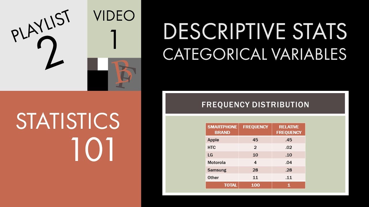
- 🔢 It explains the difference between qualitative (categorical) and quantitative variables, and how to present them graphically, with qualitative variables often using bar graphs and pie charts.
- 📊 The importance of organizing data into a frequency table and then translating that into a bar graph or pie chart is highlighted for better data interpretation.
- 📉 For quantitative variables, histograms are introduced as a method to display the frequency distribution, helping to visualize the data's overall shape and identify patterns or outliers.
- 📝 The process of constructing a histogram includes choosing classes, counting individuals in each class, and then graphically representing this data without gaps or overlaps.
- 🤔 The script poses questions about data sets, such as how a class performed, and demonstrates how organizing and summarizing data can lead to more meaningful answers.
- 📏 The concept of 'range' in a data set is explained, which is the difference between the maximum and minimum values and is crucial for constructing histograms.
- 📐 The script provides a detailed example of building a histogram for a data set showing the percentage of foreign-born residents in U.S. states, illustrating the steps involved in creating a frequency table and the histogram itself.
- 📊 It outlines the steps to identify the general shape of a distribution (uniform, symmetric, right-skewed, or left-skewed) and to spot outliers within a histogram.
- 🌱 The introduction of stem plots as a quick method for small data sets to provide a snapshot of the data's distribution, which can be easily turned into a dot plot for a different visualization.
Q & A
What is the main focus of the second lesson in the provided transcript?
-The main focus of the second lesson is on descriptive statistics, specifically on graphical presentations for a dataset to start telling the statistical story and making sense of the data.
What are the two different types of variables discussed in the script?
-The two different types of variables discussed are qualitative (categorical) and quantitative.
What is a frequency distribution and why is it important?
-A frequency distribution tells us the possible values or categories a variable can take on and how often these values or categories have been observed in the dataset. It is important because it provides a summary of the data, making it easier to understand and analyze.
What is the difference between a frequency table and a bar graph in representing a frequency distribution?
-A frequency table lists the categories and their corresponding frequencies, while a bar graph visually represents these frequencies with bars, making it easier to compare the frequencies of different categories at a glance.
How is a pie chart used to represent a frequency distribution for categorical variables?
-A pie chart represents a frequency distribution by dividing the circle into sectors, where each sector's size corresponds to the relative frequency of a category, providing a visual sense of how each category compares to the overall population.
What is a histogram and how is it different from a bar graph?
-A histogram is a graphical representation used for displaying the frequency distribution of a single quantitative variable. Unlike a bar graph, which is used for categorical variables, a histogram uses continuous bars without gaps to represent the frequency of data within certain ranges or intervals.
What are the steps involved in constructing a histogram?
-The steps involved in constructing a histogram include choosing the classes (intervals), counting the frequency of data within each class, optionally converting frequencies to relative frequencies, and then drawing the histogram with the chosen classes on the x-axis and frequency on the y-axis.
What is a stem plot and how is it used for small datasets?
-A stem plot is a graphical summary for small numerical datasets where each observation is split into a stem (all digits but the last) and a leaf (the last digit). It is used to quickly visualize the distribution and overall shape of the data, similar to a histogram but simpler and quicker to construct for small datasets.
What is a dot plot and how does it relate to a stem plot?
-A dot plot is a variation of a stem plot where instead of writing the leaf values, dots are used to represent each data point. It provides the same information about the data distribution, skewness, and potential outliers as a stem plot but in a more visual format with dots.
What should one look for when analyzing a histogram?
-When analyzing a histogram, one should look for the overall shape of the distribution (symmetric, skewed right, or skewed left) and check for any outliers or data points that fall outside the general pattern of the distribution.
What is the purpose of graphical summaries like histograms and stem plots in statistical analysis?
-Graphical summaries like histograms and stem plots help in understanding the data by providing a visual representation of the distribution, making it easier to identify patterns, skewness, and potential outliers, which are crucial for further statistical analysis and decision-making.
Outlines
📚 Introduction to Descriptive Statistics
The instructor begins by introducing the topic of descriptive statistics, explaining the importance of organizing and summarizing data to tell a statistical story. The lesson focuses on the first type of variables, qualitative or categorical, and the necessity of creating a frequency distribution to understand the data. A real-world example of college algebra class grades is used to demonstrate the raw data and the challenge of interpreting it without organization. The goal is to transform the data into a meaningful frequency distribution, which will be explored in subsequent parts of the lesson.
📊 Organizing Data with Frequency Distributions and Graphs
This section delves into the process of organizing data through frequency distributions, highlighting the creation of a frequency table for a set of grades. The instructor explains how to calculate relative frequencies and the importance of these in making comparisons between different datasets. The concept is illustrated with a bar graph, providing a visual representation of the frequency distribution. The summary emphasizes the transition from raw data to organized information, facilitating better analysis and interpretation.
🎓 Educational Attainment Data and Pie Charts
The instructor presents a dataset on the educational attainment of U.S. residents aged 25 or older, using it to introduce pie charts as a method for categorical data visualization. The pie chart is constructed by calculating the degree of each sector based on relative frequencies, providing a circular representation of the data. This visual aids in understanding the proportion of the population within each educational category, offering a different perspective compared to bar graphs and frequency tables.
📈 Transitioning to Histograms for Quantitative Data
The focus shifts to quantitative variables and the use of histograms as a graphical tool for representing data. The instructor outlines the steps for constructing a histogram, emphasizing the selection of classes or intervals and the importance of avoiding gaps and overlaps. The process is distinguished from that of a bar graph, with the histogram requiring equal-length intervals for accurate frequency representation. The explanation sets the stage for a deeper exploration of histograms in the following lessons.
📉 Constructing a Histogram for Foreign-Born Residents Data
The lesson continues with a practical example of constructing a histogram using data on the percentage of foreign-born residents in U.S. states. The instructor guides through the process of determining the range of values, choosing the number of classes, and creating a frequency table. The data is then visually represented in a histogram, illustrating the distribution and allowing for the identification of patterns and potential outliers, such as California's high percentage of foreign-born residents.
🤔 Analyzing Histograms for Distribution Patterns and Outliers
In this segment, the instructor discusses how to analyze histograms to determine the shape of the distribution—whether it's uniform, symmetric, or skewed—and to identify any outliers. The importance of understanding the distribution's shape is emphasized, as it can greatly influence the interpretation of the data. The instructor also introduces the concept of stem plots as a quick method for visualizing small datasets, providing an alternative to histograms for quick insights.
📊 Stem Plots and Dot Plots for Small Datasets
The instructor concludes the lesson by explaining the creation of stem plots, which are simplified histograms for small numerical datasets. The process involves separating each data point into a stem and a leaf, arranging them in columns, and then plotting the leaves in increasing order. The resulting visual provides a quick overview of the data's distribution. Additionally, the instructor mentions dot plots, which are similar to stem plots but use dots instead of leaf values, offering another way to represent data distribution.
📘 Assignment and Preparation for Next Week's Lesson
The instructor wraps up the lesson by reminding students to complete assignment number two on MyMathLab, which should now be manageable with the knowledge gained from the lesson. The instructor also previews the next week's topics, which will involve calculations for descriptive summaries and a deeper dive into the concept of outliers. The lesson ends on a positive note, wishing students well for the semester and looking forward to the next session.
Mindmap
Keywords
💡Descriptive Statistics
💡Data Set
💡Variable
💡Frequency Distribution
💡Categorical Variable
💡Quantitative Variable
💡Bar Graph
💡Pie Chart
💡Histogram
💡Outliers
💡Stem Plot
Highlights
Introduction to Descriptive Statistics and the importance of graphical presentations for data sets.
Explanation of a data set as a collection of data values or points for a specific group and characteristic.
Differentiation between qualitative (categorical) and quantitative variables.
Discussion on the significance of frequency distribution in understanding data.
Construction of a frequency table to organize data by categories and their frequencies.
Calculation of relative frequencies to compare data sets of different sizes.
Illustration of data organization through bar graphs for categorical variables.
Use of pie charts for representing categorical data with relative frequencies.
Transition to dealing with quantitative variables and the introduction of histograms.
Steps for constructing a histogram, including choosing classes and counting intervals.
Importance of ensuring no gaps or overlaps in classes for histogram construction.
Guidelines for choosing the number of classes in a histogram, typically between 5 and 20.
Building a histogram by hand for a data set of foreign-born residents in U.S. states.
Analysis of histogram shapes to determine if they are symmetric, skewed right, or skewed left.
Identification of outliers in histograms as data points that fall outside the overall pattern.
Introduction to stem plots as a quick method for graphically summarizing small numerical data sets.
Process of creating a stem plot by separating each observation into a stem and a leaf.
Explanation of how to identify and highlight potential outliers in a data set.
Advantages of using graphical summaries like histograms and stem plots for data analysis.
Transcripts
Browse More Related Video
Statistics 101: Describing a Categorical Variable
Descriptive statistics and data visualisation. An introduction to statistics and working with data

Elementary Stats Lesson #3 A
Sample and Population in Statistics | Statistics Tutorial | MarinStatsLectures

Elementary Statistics - Chapter 2 - Exploring Data with Tables & Graphs

Elementary Stats Lesson #4
5.0 / 5 (0 votes)
Thanks for rating: