7. Confidence Intervals
TLDRThis lecture delves into the Empirical Rule and normal distributions, highlighting their prevalence in various real-world scenarios. It demonstrates generating normal distributions in Python and verifies the rule through simulations. The Central Limit Theorem is introduced, showing how sample means approximate a normal distribution regardless of the original distribution's shape. The video also explores the use of randomness in estimating pi and function integration, showcasing Monte Carlo simulations as a powerful tool for solving complex problems.
Takeaways
- 📚 The script is from a lecture, likely part of MIT OpenCourseWare, discussing the Empirical Rule and its assumptions, including a mean estimation error of zero and normally distributed errors.
- 📉 The Empirical Rule, also known as the 68-95-99.7 rule, is associated with normal distributions, which are often referred to as Gaussian distributions after the astronomer Carl Gauss.
- 🔢 Python's random library can easily generate normal distributions using the `random.gauss` function, where the mean and standard deviation are specified as arguments.
- 📈 The lecture includes a demonstration of generating a discrete approximation of a normal distribution and plotting it using histograms with weighted bins to represent relative frequencies.
- 📊 The weights in a histogram allow for adjusting the y-axis to show fractions of values in each bin rather than counts, which is useful for interpreting the distribution as a probability density function.
- 📚 The script explains that the area under the probability density function (PDF) represents the probability of a random variable falling between two values, and the importance of integration in understanding this area.
- 🧮 The `scipy.integrate.quad` function is introduced for numerical integration, which can be used to approximate the area under the PDF and verify the empirical rule for normal distributions.
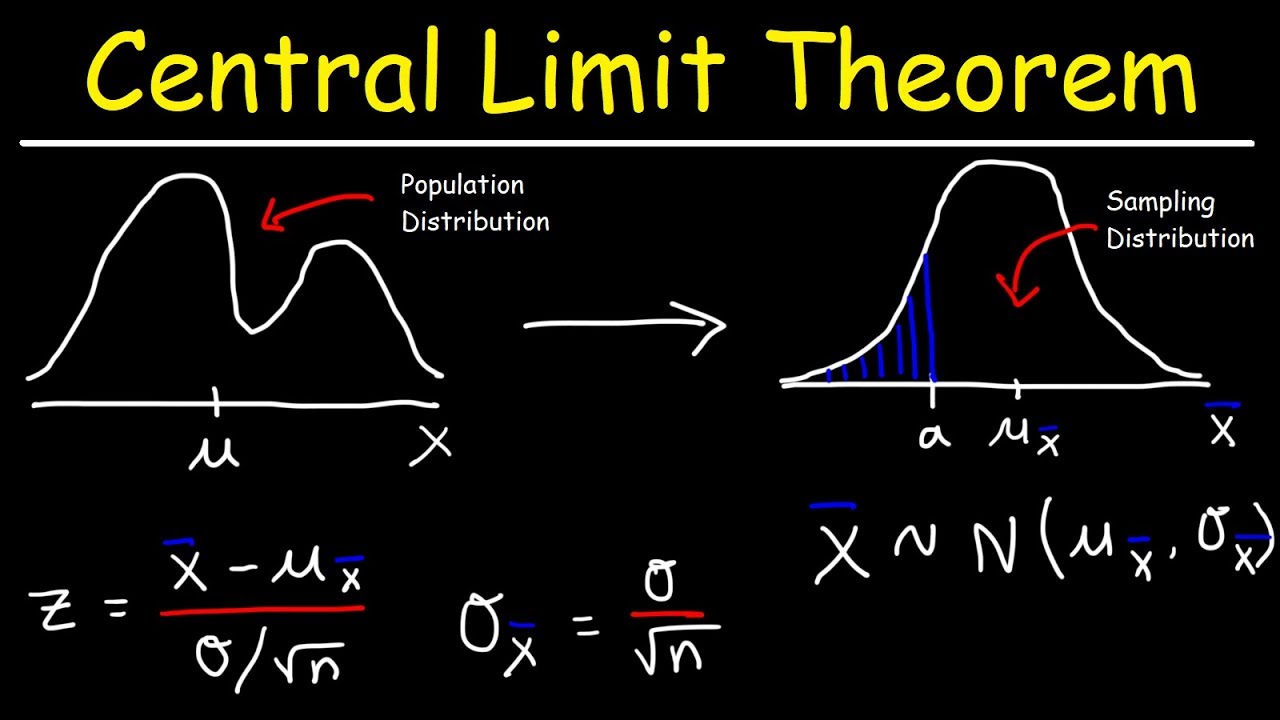
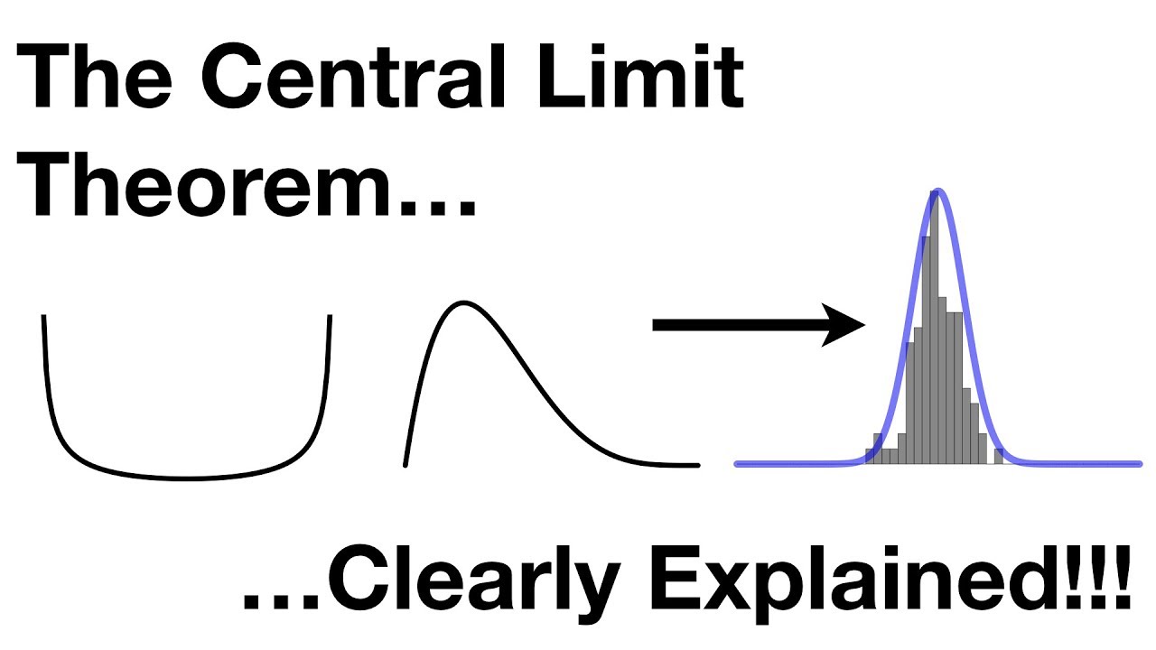
- 🎲 The Central Limit Theorem (CLT) is highlighted, stating that the means of samples from a population will be approximately normally distributed if the sample size is large enough, regardless of the population's actual distribution.
- 🃏 An example of using the CLT is given with a hypothetical continuous die, illustrating how the distribution of means approaches a normal distribution as the number of dice rolled increases.
- 🎯 The script also touches on the use of randomness and Monte Carlo simulations for estimating the value of pi, showing that randomness can be useful even in calculating deterministic values.
- 🤔 The importance of distinguishing between a statistically valid simulation and an accurate model of reality is emphasized, noting that a simulation can be reproducible but still incorrect if based on a flawed model.
Q & A
What is the Empirical Rule and what are its underlying assumptions?
-The Empirical Rule, also known as the 3-sigma rule, states that for a normal distribution, almost all data (about 99.7%) falls within three standard deviations of the mean. The assumptions are that the mean estimation error is zero and the distribution of errors is normally distributed, also referred to as Gaussian distribution.
How can normal distributions be generated in Python?
-Normal distributions can be generated in Python using the `random.gauss` function from the `random` library, where the first argument is the mean (mu) and the second argument is the standard deviation (sigma or sigma).
What is the purpose of the 'weights' argument in the 'pylab.hist' function?
-The 'weights' argument in 'pylab.hist' allows each value in the bins to be weighted differently. This can be used to adjust the y-axis to represent the fraction of values that fell in each bin rather than the count, making the histogram more interpretable.
How does the script demonstrate the application of the Empirical Rule using a Python simulation?
-The script generates a set of random values using a Gaussian distribution with a mean of 0 and a standard deviation of 100, then plots a histogram with weighted bins to show the distribution. It checks the fraction of values that fall within two standard deviations of the mean, demonstrating the Empirical Rule.
What is the formula for the Probability Density Function (PDF) of a normal distribution?
-The PDF of a normal distribution is given by the formula: \( P(x) = \frac{1}{\sigma\sqrt{2\pi}} e^{-\frac{(x-\mu)^2}{2\sigma^2}} \), where \( \mu \) is the mean and \( \sigma \) is the standard deviation.
How does the script use SciPy's 'integrate.quad' function to work with normal distribution?
-The script uses 'integrate.quad' to numerically approximate the integral of the Gaussian function over a specified range, providing an estimate of the area under the curve, which corresponds to the probability of a value falling within that range.
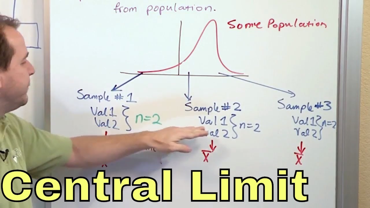
What is the Central Limit Theorem (CLT) and why is it significant?
-The Central Limit Theorem states that the distribution of sample means will be approximately normally distributed if the sample size is sufficiently large, regardless of the shape of the population distribution. It is significant because it allows the application of the empirical rule to estimate confidence intervals for the mean, even when the underlying distribution is not normal.
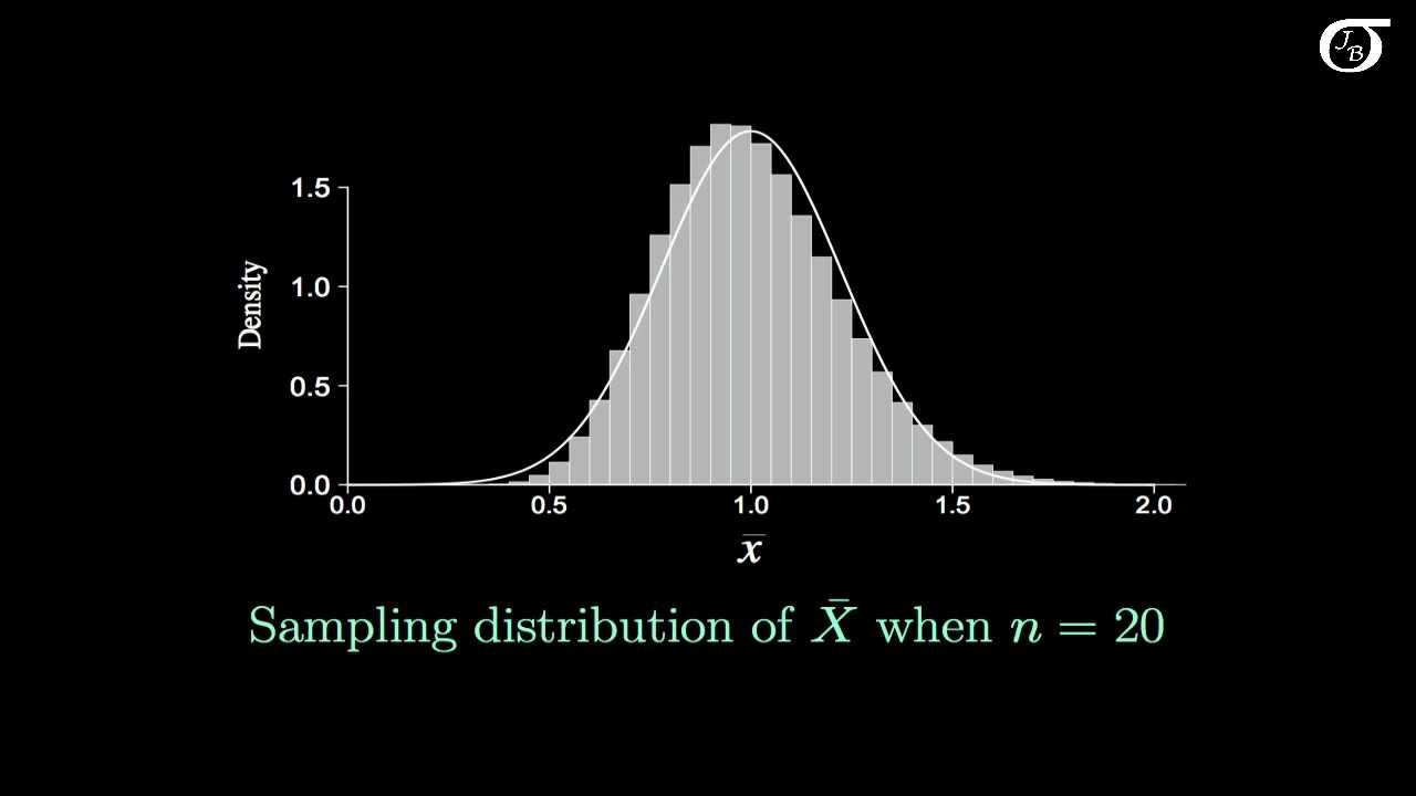
How does the script illustrate the Central Limit Theorem using a simulation of rolling dice?
-The script simulates rolling a continuous 'die' multiple times, calculates the means of these rolls for different sample sizes, and plots the distribution of these means. As the sample size increases, the distribution of means becomes more normally distributed, illustrating the CLT.
What is the Monte Carlo simulation method and how is it used to estimate the value of pi?
-The Monte Carlo simulation method is a technique that uses randomness to compute numerical results. In the context of estimating pi, it involves randomly throwing 'needles' (or points) into a square inscribed with a circle, and using the ratio of needles that fall inside the circle to those that fall within the square to estimate pi.
How does the script demonstrate the use of randomness in estimating the value of pi?
-The script presents a Python simulation where needles are 'thrown' at random within a square inscribed with a circle. The ratio of needles that fall within the circle to those in the square is used to estimate pi, demonstrating how randomness can be harnessed for a deterministic calculation.
What is the importance of understanding the difference between statistical validity and true accuracy in simulations?
-Statistical validity refers to the reliability and reproducibility of a simulation's results, while true accuracy refers to the simulation's correctness in representing reality. Understanding this difference is crucial because a statistically valid simulation can still produce inaccurate results if the model itself is flawed.
Outlines
📚 Introduction to MIT OpenCourseWare and the Empirical Rule
The video script begins with an introduction to MIT OpenCourseWare, highlighting its mission to provide free, high-quality educational resources. Viewers are encouraged to donate to support this initiative and explore additional course materials on the website. The lecture then dives into a review of the Empirical Rule, also known as the 3-sigma rule, which is based on the assumptions that the mean estimation error is zero and that errors are normally distributed, a distribution named after Carl Gauss. The script explains how to generate normal distributions in Python using the 'random.gauss' function, emphasizing the mean (mu) and standard deviation (sigma) as key parameters, and demonstrates plotting these distributions using histograms and weights to adjust the y-axis for better interpretation.
📈 Exploring Histograms, Weights, and the Empirical Rule
This paragraph delves deeper into the use of histograms to visualize data distribution, explaining how 'pylab.hist' creates histograms and the role of 'bins' in determining the number of bins. It introduces the concept of 'weights' in histograms, which allows for adjusting the significance of each bin's count, thus affecting the y-axis scale. The script demonstrates how to calculate the fraction of values falling within two standard deviations of the mean, effectively checking the validity of the Empirical Rule. The results show a discrete approximation of a probability density function, with over 95% of values within two standard deviations, aligning with the rule's expectations, albeit slightly higher due to the finite sample size and the actual magic number being 1.96 instead of 2.
📊 Probability Density Functions (PDFs) and Normal Distribution
The script transitions into a discussion about Probability Density Functions, which define the probability of a random variable falling between two values. It contrasts the smooth curve of a PDF with the jagged histogram from the previous section, emphasizing that the area under the PDF curve represents the probability. The normal distribution's PDF is introduced, along with a Python implementation that calculates the density for given values of x, mu, and sigma. The script then plots this function for a standard normal distribution (mu=0, sigma=1) over a range of x values, illustrating the distribution's shape and how it asymptotically approaches zero beyond +/-4 standard deviations.
🔢 Numerical Integration and the Central Limit Theorem (CLT)
The script introduces numerical integration techniques, specifically focusing on SciPy's 'integrate.quad' function, which approximates integrals using a numerical method called quadrature. It explains the function's parameters, including the function to integrate, limits of integration, and additional arguments for functions with more than one variable. The script demonstrates how to use this function to verify the empirical rule for normal distributions by integrating the Gaussian function over various ranges of standard deviations, confirming that the rule holds true regardless of the specific values of mu and sigma.
🎲 The Central Limit Theorem and Its Applications
This section of the script discusses the Central Limit Theorem, which states that the distribution of sample means will be approximately normal, regardless of the original distribution's shape, given a sufficiently large sample size. It explains the theorem's implications for the mean and variance of the sample means and provides examples of normal distributions in real-world data, such as SAT scores, oil price changes, and human heights. The script also contrasts these with the uniform distribution of a roulette wheel's outcomes, highlighting the difference between single-event probabilities and the mean of multiple events.
👁️ Exploring the Central Limit Theorem with a Continuous Die
The script presents a thought experiment involving a continuous die that yields real numbers between 0 and 5, rather than discrete integers. It simulates rolling this die multiple times to demonstrate the Central Limit Theorem in action. As the number of dice rolled increases, the distribution of their means becomes increasingly normal, even though the individual outcomes are not normally distributed. This simulation visually illustrates the theorem's effectiveness and the emergence of a normal distribution for the means of samples.
🃏 Monte Carlo Simulations and the Value of Pi
The script shifts focus to the use of randomness in computing non-random quantities, such as the value of pi, through Monte Carlo simulations. It recounts historical methods of estimating pi, from the Egyptians and the Bible to Archimedes' polygon approach. The French mathematicians Buffon and Laplace are highlighted for proposing a method that involves dropping needles at random onto a surface inscribed with a circle, using the ratio of needles landing inside the circle to estimate pi. The script describes a class simulation involving a blindfolded archer shooting arrows as a modern take on this method.
🎯 Monte Carlo Simulation for Estimating Pi
This paragraph details the implementation of a Monte Carlo simulation to estimate the value of pi. It outlines the process of simulating the needle-drop experiment by generating random points and calculating the ratio of points within the circle to those in the square. The script explains how to iteratively increase the number of trials and calculate the mean and standard deviation of the estimates to achieve a desired precision. It emphasizes the importance of not only obtaining a good estimate but also being able to confidently assert that the estimate is close to the true value.
🤔 The Limitations of Simulations and Statistical Validity
The script concludes with a cautionary note about the limitations of simulations and the difference between statistical validity and truth. It points out that while a simulation can provide confidence in an estimate's reproducibility, it cannot guarantee the accuracy of the model itself. This is illustrated by introducing a deliberate error in the simulation's formula, which results in confidence intervals for an incorrect value of pi. The importance of sanity checks and validating the simulation model against known values or expectations is underscored to ensure the reliability of the results.
🔧 Wrapping Up and Future Topics
In the final paragraph, the script wraps up the discussion on estimating pi and the use of randomness in simulations. It summarizes the technique for estimating the area of any region by using an enclosing region with a known area and random points to determine the fraction that falls within the desired region. The script also briefly mentions the application of this technique to integration, providing an example with the sine function. It concludes by informing viewers that a different topic will be covered in the next lecture.
Mindmap
Keywords
💡Empirical Rule
💡Gaussian Distribution
💡Histogram
💡Weights
💡Probability Density Function (PDF)
💡Integration
💡Central Limit Theorem (CLT)
💡Monte Carlo Simulation
💡Standard Deviation
💡Confidence Interval
Highlights
Introduction to the Empirical Rule and its underlying assumptions, including mean estimation error being zero and normal distribution of errors.
Explanation of the Gaussian distribution named after Carl Gauss, and its characteristics.
Demonstration of generating normal distributions in Python using the random library's gauss function.
Use of histogram bins, weights, and the significance of the weights in altering the y-axis interpretation in data visualization.
Illustration of the empirical rule through a Python-generated plot showing the distribution of errors and their relation to the mean.
Introduction to Probability Density Functions (PDFs) and their role in defining the probability of a random variable lying between two values.
Coding implementation of a normal distribution PDF and its plot to visualize the distribution curve.
Clarification on the difference between a probability density function and actual probabilities, emphasizing the area under the curve.
Introduction to the SciPy library and its integrate.quad function for numerical integration of functions.
Practical application of the empirical rule in various real-world scenarios such as SAT scores and oil price changes.
Discussion on the limitations of the empirical rule with examples like the spins of a roulette wheel not following a normal distribution.
Explanation of the Central Limit Theorem (CLT) and its implications for the distribution of sample means.
Simulation of rolling a 'continuous die' to demonstrate the CLT and the emergence of a normal distribution in sample means.
Use of Monte Carlo simulations to estimate the value of pi, showcasing the power of randomness in computing non-random quantities.
Execution of a Monte Carlo simulation in Python to estimate pi, including the calculation of standard deviation for confidence intervals.
The importance of distinguishing between a statistically valid simulation and an accurate model of reality, with a cautionary note on potential bugs.
General technique for estimating areas of regions and integrating functions using randomness, highlighting the broad applicability of simulation methods.
Transcripts
Browse More Related Video

Central limit theorem | Inferential statistics | Probability and Statistics | Khan Academy

Sampling distribution of the sample mean | Probability and Statistics | Khan Academy
Introduction to the Central Limit Theorem
Central Limit Theorem - Sampling Distribution of Sample Means - Stats & Probability
02 - What is the Central Limit Theorem in Statistics? - Part 1
The Central Limit Theorem, Clearly Explained!!!
5.0 / 5 (0 votes)
Thanks for rating: