Lec 33 | MIT 18.01 Single Variable Calculus, Fall 2007
TLDRThis MIT OpenCourseWare lecture delves into polar coordinates, focusing on calculating areas and exploring variable 'pies' with radii dependent on theta. Professors illustrate the area calculation with pie slices and introduce the formula for differential area, 1/2 r^2 d theta. They also discuss the implications of polar coordinates in astronomy, such as Kepler's Law and conservation of angular momentum, highlighting the physical relevance of polar coordinate representation. The lecture includes examples, such as calculating the area of a circle with r = 2a cos(theta) and plotting polar graphs like r = sin(2theta), which forms a four-leaf rose. The professor also covers the conversion from polar to rectangular coordinates and provides insights into exam topics, emphasizing integration techniques and the importance of setup in integrals.
Takeaways
- 📚 The lecture continues the discussion on polar coordinates, focusing on the concept of area in polar coordinates, which was not covered in the previous session.
- 🍰 The professor uses the analogy of a pie to explain the area in polar coordinates, defining the area of a slice as 'delta A' and relating it to the radius 'a' and arc length 'delta theta'.
- 📉 For a pie with a variable radius (r = r(theta)), the area under a curve is calculated by integrating 1/2 * r^2 d theta over the desired interval, which is applicable when 'r' is a function of 'theta'.
- 🔄 The class revisits the example r = 2a cos(theta), which represents a circle, and the professor demonstrates how to calculate the area by integrating from -pi/2 to pi/2.
- 📈 The professor emphasizes the importance of understanding the range of integration by visualizing or using formulas, rather than guessing, to avoid errors in calculating areas.
- 📝 The lecture includes a review of trigonometric integrals, specifically using a double angle formula to simplify and solve integrals involving cos^2(theta).
- 🌐 The professor discusses the implications of integrating over a full circle (0 to 2pi), noting that it would double the area and is not typically desired unless explicitly calculating the entire region.
- 🌹 The concept of plotting polar functions is explored with examples like r = sin(2theta), which results in a four-leaf rose pattern, highlighting the importance of visual understanding.
- 📉 The lecture introduces the function r = 1/(1 + 2cos(theta)) and discusses its plot, which resembles a hyperbola with branches on either side of the origin, and its relevance to astronomy and Kepler's Law.
- ⚖️ The professor connects the polar area formula to physical concepts like angular momentum conservation and Kepler's Law, showing the formula's importance in describing the motion of celestial bodies.
- 📝 The lecture concludes with a review of exam topics, emphasizing techniques of integration, parametric curves, arc length, area of surfaces of revolution, and polar coordinates, with a reminder that the exam will cover these areas.
Q & A
What is the main topic discussed in the video script?
-The main topic discussed in the video script is polar coordinates, with a focus on the calculation of areas in polar coordinates and the connection to astronomical applications like Kepler's Law.
What is the basic formula for the area of a slice in polar coordinates?
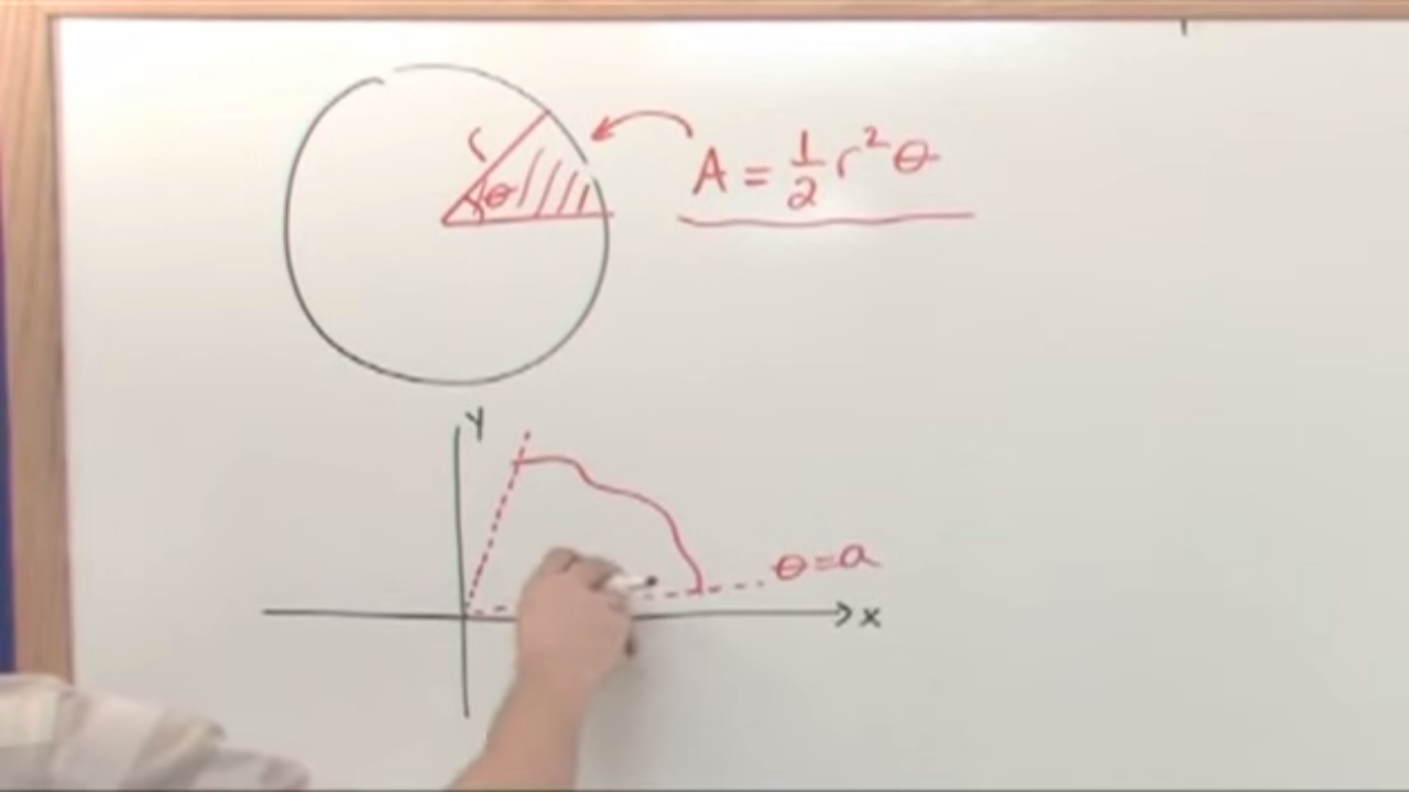
-The basic formula for the area of a slice in polar coordinates is delta A = 1/2 * a^2 * delta theta, where 'a' is the radius and 'delta theta' is the angular change.
How does the professor illustrate the concept of area in polar coordinates using a pie?
-The professor uses the analogy of a pie and its slice to explain the concept of area in polar coordinates. The pie represents the whole area, and a slice with an arc length of delta theta represents a small portion of the area, delta A.
What is the integral formula for the total area of a variable pie with radius r(theta)?
-The integral formula for the total area of a variable pie with radius r(theta) is the integral from some starting place to some end place of 1/2 * r^2 d theta.
Can you explain the example given in the script involving the polar equation r = 2a cos(theta)?
-The example r = 2a cos(theta) represents a circle in polar coordinates. The area enclosed by this equation between -pi/2 and pi/2 is calculated by integrating 1/2 * (2a cos(theta))^2 with respect to theta, which results in pi * a^2, the area of the circle.
What is the significance of the point (0, 0) in polar coordinates as explained in the script?
-The point (0, 0) in polar coordinates is significant as it represents the center of the universe from the point of view of the problem. It is the reference point, similar to the center of a radar screen, around which all other points are defined.
How does the script discuss the plotting of polar coordinates outside the range of theta = pi/2?
-The script discusses that when plotting polar coordinates outside the range of theta = pi/2, the radius r can become negative, causing the plot to go backward. This results in the curve sweeping around the same circle multiple times, which can lead to over-counting the area if not accounted for properly.
What is a four-leaf rose in the context of the script?
-A four-leaf rose is a shape plotted from the polar equation r = sin(2theta). It has four distinct 'leaves' due to the symmetry of the sine function, each corresponding to a quadrant in polar coordinates.
What is the connection made in the script between polar coordinates and astronomical observations?
-The script connects polar coordinates to astronomical observations by discussing Kepler's Law, which states that the rate of change of area swept out by a celestial body (like a comet) relative to the sun is constant. This is related to the polar formula for area and the conservation of angular momentum.
How does the script address the topic of integration techniques in the exam?
-The script addresses integration techniques by stating that three main techniques will be tested: trig substitution, integration by parts, and partial fractions. It also mentions that if a particular integral is too complex, the professor may provide a hint or advise not to attempt it.
Outlines
📚 Introduction to Polar Coordinates and Area Calculation
The professor begins by introducing the topic of polar coordinates, focusing on the concept of area in polar coordinates. Using the analogy of a pie, the professor explains how to calculate the area of a slice (delta A) with a radius 'a' and an arc length delta theta. The formula for the area of the pie is given as pi * a^2, and the area of the slice is derived as 1/2 * a^2 * delta theta. The lecture then transitions into discussing the area of a 'variable pie' where the radius r is a function of the angle theta (r = r(theta)), and the method of subdividing the pie into small chunks to calculate the total area is introduced.
🔍 Detailed Discussion on Variable Radius and Area Calculation
The professor delves deeper into the concept of a variable radius in polar coordinates, using the example of a pie with a 'wavy crust'. The idea is to break down the area into small, manageable slices, each with a circular arc. The approximation for the area of each slice, delta A, is given as approximately 1/2 * r^2 * delta theta, with the exact formula being derived from the limit as the slices become infinitesimally small. The total area is then expressed as the integral from a starting angle to an ending angle of 1/2 * r^2 d theta. The professor emphasizes that this formula is particularly useful when r is a function of theta.
📘 Example Calculation of Area for a Circle in Polar Coordinates
An example is presented to illustrate the calculation of the area for a circle in polar coordinates, using the equation r = 2a * cos(theta). The professor explains that the area is only swept out between -pi/2 and pi/2 due to the cosine function being positive in this range and becoming zero at the endpoints. The integral to calculate the area is set up and solved, resulting in pi * a^2, which is the expected area of a circle. The professor also addresses questions from students regarding the determination of the range for integration and the visualization of the polar curve.
📙 Exploring the Effects of Theta Range on Polar Coordinates Plotting
The professor discusses what happens outside the range of theta for polar coordinates plotting, specifically beyond pi/2. Using the elbow analogy, the professor explains that as theta increases beyond pi/2, the radius r becomes negative, effectively causing the plot to go backward. It is emphasized that the plot will sweep out the same region twice, which could lead to double counting of the area if the integration range is extended to 2pi or beyond. The professor also addresses the possibility of integrating from 0 to pi, which surprisingly yields the correct area but through a less conventional approach.
🌿 Plotting and Understanding Polar Functions: The Four-Leaf Rose
The professor provides a detailed walkthrough of plotting the polar function r = sin(2theta), which results in a shape known as a four-leaf rose. By plotting key points at theta = 0, pi/4, and pi/2, the professor demonstrates how the function behaves symmetrically in all quadrants. The importance of understanding the order of plotting is highlighted to grasp the overall shape and behavior of the polar function.
📒 Plotting and Analyzing a Complex Polar Function
The professor introduces a more complex polar function, r = 1 / (1 + 2cos(theta)), and begins by plotting several points to understand its behavior. Key points are identified at theta = 0, pi/2, and -pi/2, revealing that the function has a denominator of zero at certain angles, indicating asymptotes. The professor then transitions into discussing the conversion of polar coordinates to rectangular coordinates, which is essential for further analysis of the function's shape and characteristics.
📉 Transitioning from Polar to Rectangular Coordinates and Hyperbolic Trajectories
The professor demonstrates the conversion of the polar function r = 1 / (1 + 2cos(theta)) into its rectangular coordinate form, resulting in an equation that represents a hyperbola. The connection between the polar formula for area and Kepler's Law in astronomy is highlighted, showing how the rate of change of area swept out by a comet's trajectory around the sun is constant. This leads to a discussion on the conservation of angular momentum and its physical implications, such as the effect on spinning objects.
🎯 Integration Techniques and Exam Preparation
The professor outlines the topics that will be covered in the upcoming exam, emphasizing three main integration techniques: trig substitution, integration by parts, and partial fractions. The second half of the exam will focus on parametric curves, arc length, area of surfaces of revolution, and polar coordinates, including area calculations. The professor provides guidance on exam preparation, advising students on which techniques to apply and when to seek assistance or avoid particular problems.
📌 Advanced Integration Techniques and Partial Fractions
The professor discusses advanced topics in integration, specifically focusing on partial fractions and how to handle them when the denominator contains repeated factors or higher-degree terms. The importance of setting up the integral correctly and knowing when to use long division or other algebraic methods is emphasized. The professor also addresses the potential complexity of integration by parts and the use of reduction formulas, advising students on how to approach these techniques during the exam.
🧩 Integration by Parts and Handling Tricky Integrals
The professor provides an example of using integration by parts for a complex integral involving a function that simplifies upon differentiation. The steps of the process are outlined, including the correct identification of u and v', and the subsequent steps to solve the integral. The professor also introduces a shortcut for handling cases where the numerator and denominator are closely related, demonstrating how to simplify the integral and arrive at the final solution.
Mindmap
Keywords
💡Polar Coordinates
💡Area
💡Delta Theta
💡Riemann Sums
💡Integral
💡Cosine
💡Variable Pie
💡Hyperbola
💡Kepler's Law
💡Angular Momentum
Highlights
Introduction to polar coordinates and their application in calculating areas, using the analogy of a pie to explain the concept.
Explanation of the formula for the area of a sector in polar coordinates, delta A = 1/2 a^2 delta theta.
Transition to variable pies with crusts that vary, represented by r = r(theta), and the method to calculate their areas.
Discussion on the approximation of area in polar coordinates using Riemann sums and the limit concept.
Derivation of the main formula for the area in polar coordinates when r is a function of theta, involving integration.
Example problem involving the calculation of the area for a circle using polar coordinates, with r = 2a cos(theta).
Clarification on determining the range for integration in polar coordinates through geometric interpretation and formulas.
Integration technique review, specifically using double angle formulas for trigonometric integrals.
Demonstration of the process to calculate the area of a circle using trigonometric integrals and obtaining pi*a^2.
Illustration of the geometric interpretation of polar coordinates and how to visualize the range of theta.
Discussion on the implications of integrating over a full circle (0 to 2pi) and the potential for double counting areas.
Introduction of the concept of plotting polar coordinates and the effect of theta values beyond pi/2.
Explanation of the behavior of polar functions, like r = sin(2theta), and their corresponding graphical representations.
Description of the four-leaf rose pattern generated by the polar function r = sin(2theta) and its significance.
Introduction and plotting of the polar function r = 1/(1 + 2cos(theta)) and its asymptotic behavior.
Conversion of polar coordinates to rectangular coordinates and the identification of the curve as a hyperbola.
Connection between polar coordinates, hyperbolic trajectories, and Kepler's Law in astronomy.
Discussion on the physical interpretation of the rate of change of area in polar coordinates and its relation to angular momentum conservation.
Overview of exam topics including techniques of integration, parametric curves, arc length, and area in polar coordinates.
Advice on exam preparation, specifically regarding the decision on which integration technique to apply for complex integrals.
Explanation of partial fraction decomposition, especially for handling repeated factors and setting up coefficients.
Demonstration of an advanced integration technique involving integration by parts and handling of complex integrands.
Transcripts
Browse More Related Video
Double Integrals in Polar Coordinates
Lesson 15 - Area And Length In Polar Coordinates (Calculus 2 Tutor)
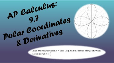
AP Calculus BC Lesson 9.7
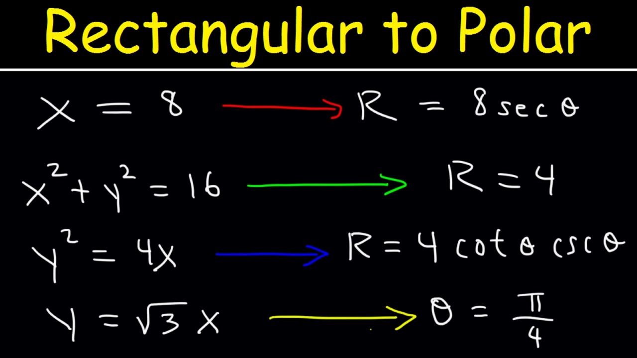
Rectangular Equation to Polar Equations, Precalculus, Examples and Practice Problems
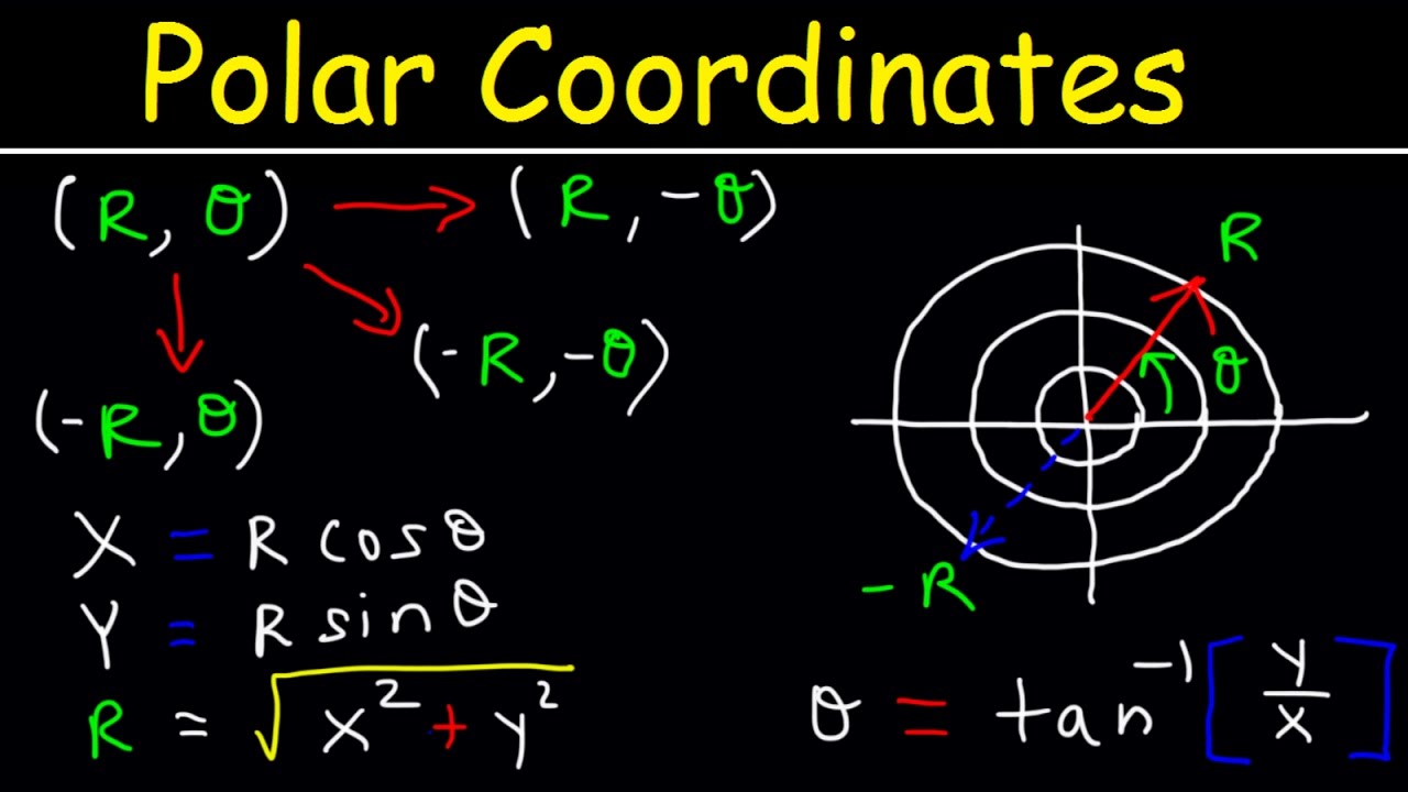
Polar Coordinates Basic Introduction, Conversion to Rectangular, How to Plot Points, Negative R Valu
Polar coordinates 2 | Parametric equations and polar coordinates | Precalculus | Khan Academy
5.0 / 5 (0 votes)
Thanks for rating: