Analyzing concavity (algebraic) | AP Calculus AB | Khan Academy
TLDRThe video script discusses the concept of concavity in the context of a fourth-degree polynomial function, denoted as 'g'. It explains that concave upward intervals are where the slope increases, resembling an upward-opening U shape, while concave downward intervals show a decreasing slope. The presenter guides through the process of finding the first and second derivatives of 'g' to determine these intervals. By setting the second derivative to zero, critical points at x = ±1 are identified, which divide the number line into intervals for analysis. Testing values within these intervals reveals that the function is concave downward from negative infinity to -1 and from 1 to infinity, and concave upward between -1 and 1. The script concludes with a graph that visually confirms these findings, demonstrating how derivatives can reveal a function's concavity without needing to graph it.
Takeaways
- 📚 The function g is a fourth-degree polynomial, and we are interested in its concavity over different intervals.
- 🔍 Concave upwards means the slope is increasing, resembling an upward-opening U shape, which corresponds to the first derivative increasing and the second derivative (g'') being greater than zero.
- 🔍 Concave downwards means the slope is decreasing, which corresponds to the first derivative decreasing and the second derivative (g'') being less than zero.
- 🧮 To find the intervals of concavity, we need to calculate the second derivative of g and look for points where it changes sign (from positive to negative or vice versa).
- 📈 The first derivative of g, denoted as g'(x), is calculated using the power rule and consists of terms involving x cubed and x to the first power.
- 📉 The second derivative of g, denoted as g''(x), simplifies to -12x squared plus 12, which is a quadratic expression.
- 🔧 The second derivative g''(x) is undefined for no x values, so we focus on where it equals zero to find potential transition points for concavity.
- 🔑 Setting g''(x) to zero and solving gives x equal to plus or minus one, which are the critical points for concavity transitions.
- 📍 By testing values in the intervals (e.g., x = -2, 0, 2), we determine the sign of g''(x) and thus the concavity over the intervals (-∞, -1), (-1, 1), and (1, ∞).
- 📉 For x < -1 and x > 1, g''(x) is negative, indicating the function is concave downward in these intervals.
- 📈 For -1 < x < 1, g''(x) is positive, indicating the function is concave upward in this interval.
- 📊 A graph of the function g and its derivatives confirms the analytical findings, showing the correct intervals of concavity.
Q & A
What is the main topic discussed in the video script?
-The main topic discussed in the video script is the concept of concavity for a fourth-degree polynomial function, specifically how to determine the intervals over which the function is concave upwards or downwards.
What does it mean for a function to be concave upwards?
-A function is concave upwards over an interval where the slope is increasing. This means that the first derivative is increasing, and the second derivative is greater than zero.
What does it mean for a function to be concave downwards?
-A function is concave downwards over an interval where the slope is decreasing. This implies that the first derivative is decreasing, and the second derivative is less than zero.
What is the first step in determining the concavity of a function?
-The first step in determining the concavity of a function is to find its first derivative, which represents the slope of the function.
What is the second step in determining the concavity of a function?
-The second step is to find the second derivative of the function. The sign of the second derivative indicates whether the function is concave upwards or downwards.
What is the significance of the second derivative being equal to zero?
-The second derivative being equal to zero indicates a point where the concavity might change, either from concave upwards to downwards or vice versa.
How does the sign of the second derivative relate to the concavity of a function?
-If the second derivative is positive, the function is concave upwards. If it is negative, the function is concave downwards.
What is the process for finding the intervals of concavity for the given function g(x)?
-The process involves taking the second derivative of g(x), setting it equal to zero to find critical points, and then testing intervals around these points to determine where the second derivative is positive or negative.
What is the role of the number line in determining the intervals of concavity?
-The number line is used to visually represent the intervals around the critical points where the concavity changes, helping to identify where the function is concave upwards or downwards.
How does the video script demonstrate the concavity of the function without graphing?
-The script demonstrates concavity by analyzing the sign of the second derivative in different intervals and explaining the implications of these signs on the shape of the function.
What is the final step in the script's process to confirm the concavity intervals?
-The final step is to graph the function and visually confirm that the intervals determined through algebraic methods match the observed concavity on the graph.
Outlines
📚 Understanding Concavity of a Fourth Degree Polynomial
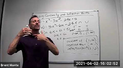
The first paragraph introduces the concept of concavity for the function g, which is a fourth degree polynomial. The voiceover explains that concave upwards means the slope is increasing, resembling an upward opening U, while concave downwards indicates a decreasing slope. The explanation includes the relationship between the first and second derivatives: a positive second derivative (g''(x) > 0) implies concave upwards, and a negative second derivative (g''(x) < 0) implies concave downwards. The process involves finding the second derivative of g and identifying points where it changes sign, which are critical in determining the intervals of concavity. The first derivative, g'(x), is calculated using the power rule, and the second derivative, g''(x), is derived from g'(x). The critical points where the second derivative is zero are found by solving the equation -12x^2 + 12 = 0, which simplifies to x^2 = 1, giving x = ±1. These points divide the graph into intervals that need to be analyzed for concavity.
📉 Analyzing the Intervals of Concavity for the Polynomial Function
The second paragraph delves into determining the concavity of the polynomial function g by examining the sign of the second derivative across different intervals. The intervals considered are from negative infinity to -1, between -1 and 1, and from 1 to infinity. By testing values within these intervals, it's established that the function is concave downwards for x < -1 and x > 1, as the second derivative g''(x) is negative in these regions. Specifically, g''(-2) and g''(2) both equal -36, indicating concave downwards. For the interval between -1 and 1, the second derivative is positive, as demonstrated by g''(0) = 12, confirming that the function is concave upwards in this range. The paragraph concludes with a visual confirmation by graphing the function, showing that the analytical findings about concavity align with the graph's shape, thus validating the earlier algebraic deductions.
Mindmap
Keywords
💡Concave Upward
💡Concave Downward
💡First Derivative
💡Second Derivative
💡Polynomial
💡Intervals
💡Slope
💡Power Rule
💡Critical Points
💡Quadratic Expression
💡Graph
Highlights
Introduction to the concept of concavity and its significance in understanding the behavior of a function.
Explanation of concave upwards as an interval where the slope is increasing.
Illustration of concave upwards using an upward opening U shape.
Description of how the slope changes from negative to positive in a concave upwards interval.
Connection between first and second derivatives in determining concavity.
Criteria for concave upwards: second derivative greater than zero.
Introduction to concave downwards as the opposite of concave upwards.
Explanation of concave downwards as an interval where the slope is decreasing.
Criteria for concave downwards: second derivative less than zero.
Methodology to find intervals of concavity by analyzing the second derivative.
Application of the power rule to find the first derivative of a fourth degree polynomial.
Derivation of the second derivative of the given function g.
Identification of points where the second derivative is undefined or zero.
Solution for x when the second derivative equals zero.
Analysis of the concavity on intervals defined by the roots of the second derivative.
Graphical representation of the concavity intervals on a number line.
Testing the concavity on specific intervals using the second derivative.
Conclusion of concave downward intervals from negative infinity to -1 and from 1 to infinity.
Conclusion of the concave upward interval between -1 and 1.
Verification of concavity findings with a pre-graphed function.
Demonstration of the practical application of derivatives to understand function behavior without graphing.
Transcripts


5.0 / 5 (0 votes)
Thanks for rating: