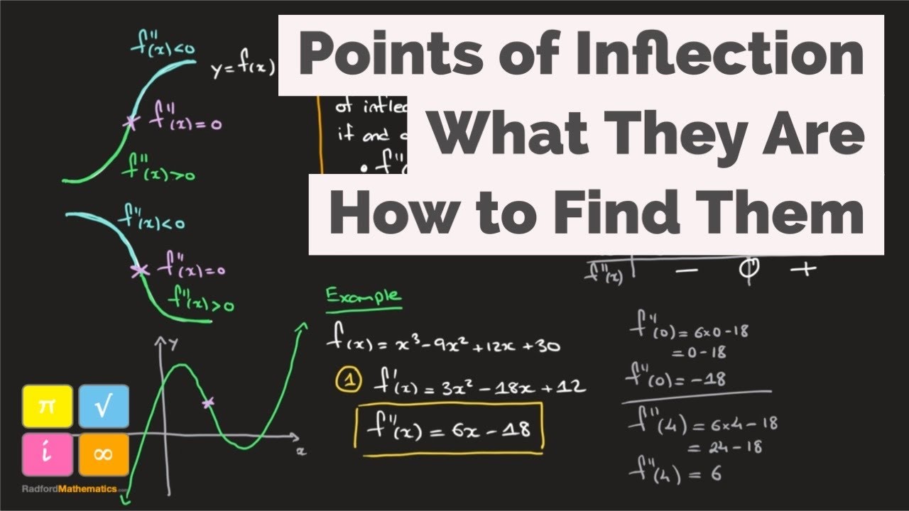
Learn how to find the points of inflection for an equation
TLDRThe video transcript details a mathematical lesson on finding intervals of concavity and points of inflection for a given function. The instructor opts to use the power rule to find the first derivative and then the product rule for the second derivative. After simplifying the second derivative, the focus shifts to identifying points of inflection by setting the numerator to zero, leading to the discovery of x = ±1 as potential points. The instructor then sets up a table to test the sign of the second derivative in intervals around these points, concluding that the function is concave up on (-∞, -1) ∪ (1, ∞) and concave down on (-1, 1). The process is methodical, emphasizing the importance of understanding when the second derivative changes sign to determine concavity.
Takeaways
- 🔍 The goal is to find intervals of concavity and values of inflection for a given function.
- 📚 The process starts by finding the second derivative of the function, which is done by first finding the first derivative.
- 👉 The power rule is suggested for finding the first derivative, but the chain rule is also applicable.
- 🤔 The instructor contemplates using the quotient rule but opts for the product rule for the second derivative.
- 📝 The second derivative is calculated with a focus on simplifying the expression and finding a common denominator.
- 🧐 The second derivative is simplified to \( \frac{36x^2 - 36}{(x^2 + 3)^3} \) and further to \( \frac{x^2 - 1}{(x^2 + 3)^3} \).
- 🚫 The second derivative is never undefined as the denominator cannot be zero in the real number system.
- ✂️ The numerator is set to zero to find the potential points of inflection, resulting in \( x = \pm1 \).
- 📉 A table is set up to test the sign of the second derivative at points around \( x = -1 \) and \( x = 1 \) to determine concavity.
- 📈 The function is found to be concave up on the intervals \( (-\infty, -1) \) and \( (1, \infty) \) and concave down on the interval \( (-1, 1) \).
- 📌 Points of inflection are confirmed at \( x = -1 \) and \( x = 1 \) where the concavity changes from positive to negative and vice versa.
Q & A
What is the main objective of the example discussed in the transcript?
-The main objective is to find the intervals of concavity and the values of inflection for a given function.
What method is suggested for finding the second derivative in the transcript?
-The power rule is suggested for finding the first derivative, and then the product rule is used for finding the second derivative.
Why is the quotient rule not preferred in this example?
-The quotient rule is not preferred because it is more complex and the problem can be simplified using the product rule.
What is the first step in finding the second derivative according to the transcript?
-The first step is to find the first derivative, which can be done by applying the power rule.
How is the chain rule mentioned in the transcript?
-The chain rule is mentioned as a potential method but is not used in this example, as the power rule is applied instead.
What is the process for finding the second derivative in the transcript?
-The process involves rewriting the first derivative into a form that can be differentiated again using either the product or quotient rule, and then applying the product rule to find the second derivative.
What is the significance of the second derivative in the context of concavity and inflection points?
-The second derivative is significant because points of inflection occur where the second derivative is either equal to zero or undefined, and it helps determine the intervals of concavity.
How does the transcript handle the possibility of the second derivative being undefined?
-The transcript checks for values that would make the denominator of the second derivative equal to zero, concluding that there are no real numbers that would make it undefined.
What is the method used to find the points of inflection in the transcript?
-The method involves setting the numerator of the second derivative equal to zero and solving for x to find the points of inflection.
How does the transcript determine the intervals of concavity?
-The transcript determines the intervals of concavity by evaluating the sign of the second derivative in different intervals around the points of inflection.
What is the conclusion about the concavity of the function in the transcript?
-The conclusion is that the function is concave up on the intervals (-∞, -1) and (1, ∞) and concave down on the interval (-1, 1).
Outlines
📚 Calculus: Finding Intervals of Concavity and Points of Inflection
This paragraph introduces a calculus problem focused on determining the intervals of concavity and points of inflection for a given function. The speaker opts to find the second derivative, initially considering the quotient rule but then choosing the power rule for simplicity. The process involves differentiating the function twice, with the first derivative using the power rule and the second derivative employing the product rule. The resulting second derivative is simplified and factored to prepare for finding the points of inflection, which are identified when the second derivative is zero or undefined. The speaker clarifies that there are no undefined points since the denominator cannot be zero in the real number system, and then proceeds to find when the second derivative equals zero.
🔍 Analyzing the Second Derivative for Points of Inflection
In this paragraph, the focus is on setting the numerator of the second derivative to zero to find potential points of inflection, which occur at x = ±1. The speaker then constructs a table to test the sign of the second derivative around these points. By plugging in values less than -1, between -1 and 1, and greater than 1, the speaker determines the concavity of the function in different intervals. The function is found to be concave up on the intervals (-∞, -1) and (1, ∞) and concave down on the interval (-1, 1). The points x = -1 and x = 1 are confirmed as points of inflection where the function changes concavity. The summary concludes with a clear distinction between these points and other mathematical concepts like asymptotes, emphasizing that these are indeed points of inflection.
Mindmap
Keywords
💡Concavity
💡Inflection Point
💡First Derivative
💡Second Derivative
💡Quotient Rule
💡Power Rule
💡Chain Rule
💡Product Rule
💡Undefined
💡Common Denominator
💡Concave Up/Down Intervals
Highlights
Introduction to finding intervals of concavity and inflection points.
Choosing to use the second derivative to analyze concavity and inflection.
Avoiding the quotient rule in favor of the power rule for the first derivative.
Using the chain rule correctly to find the first derivative.
Preference for the product rule over the quotient rule for the second derivative.
Applying the product rule to find the second derivative.
Simplifying the second derivative expression.
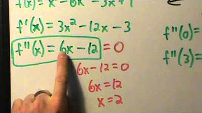
Identifying potential points of inflection by setting the second derivative to zero.
Determining that the second derivative is never undefined in the real number system.
Solving for x to find potential points of inflection at x = ±1.
Setting up a table to test the concavity intervals around the potential points of inflection.
Analyzing the sign of the second derivative to determine concavity.
Finding that the function changes concavity at x = -1 and x = 1.
Describing the intervals where the function is concave up and concave down.
Providing justification for the concavity intervals based on the sign of the second derivative.
Emphasizing the importance of distinguishing points of inflection from asymptotes.
Concluding the analysis with the correct intervals of concavity and points of inflection.
Transcripts
Browse More Related Video
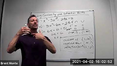
Finding Concavity and Inflection Points

Concavity, Inflection Points, and Second Derivative

Calculus I: Finding Intervals of Concavity and Inflection point
Point of Inflection - Point of Inflexion - f''(x)=0 - Definition - How to Find - Worked Example 1
Calculus I - Concavity and Inflection Points - Example 1

Inflection Point Grade 12
5.0 / 5 (0 votes)
Thanks for rating: