Geometry of the Second Derivative (1 of 4: Reviewing the Derivative)
TLDRIn this educational video script, the presenter explores the concept of a cubic function without relying on calculus. They begin by factorizing a simple cubic equation, revealing it to be a perfect square, which helps visualize the function's graph with three roots. The presenter then introduces the derivative to find stationary points, differentiating the function to locate these points more precisely. They emphasize the importance of understanding the geometry of the function, especially the location and nature of stationary points, which are crucial for sketching the function's graph accurately. The script concludes with a practical demonstration of plotting the function, including its intercepts and stationary points, providing a hands-on approach to understanding cubic functions.
Takeaways
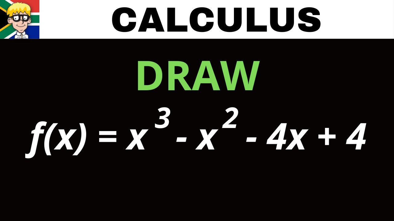
- 📚 The lesson focuses on understanding a cubic function without calculus by factorizing it.
- 🔍 The cubic function is factorized to x(x - 3)^2, which helps visualize the function's graph.
- 📈 The function has three roots, one at x = 0 and two at x = 3, indicating a repeated root.
- 📉 The leading coefficient of the cubic function is positive, suggesting the function will rise to positive infinity as x increases.
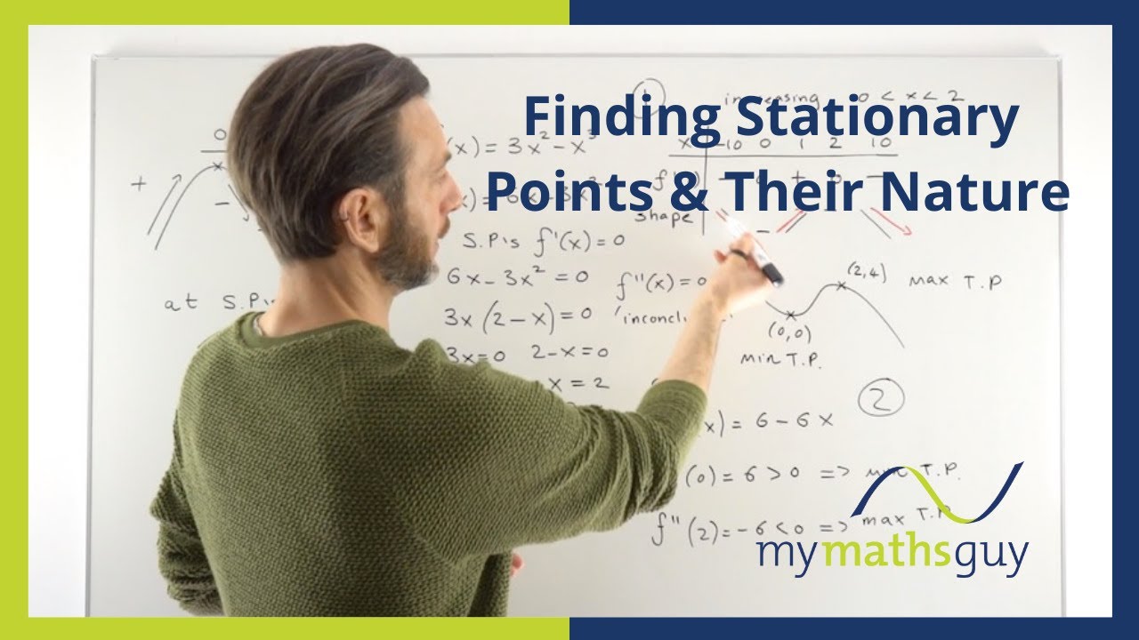
- 🔑 The derivative of the function is computed to find stationary points, which are critical for understanding the function's geometry.
- 📌 The first derivative is factorized to 3(x - 1)(x - 3), indicating stationary points at x = 1 and x = 3.
- 📐 The stationary point at x = 3 is also a root, so its y-coordinate is known to be 0.
- 📊 The y-coordinate for the stationary point at x = 1 is calculated to be 4, giving us the point (1,4).
- 📝 The teacher emphasizes the importance of differentiating between zeros (where the function equals zero) and roots (where the graph intersects the x-axis).
- 🖌️ The final graph of the function is drawn with the roots, stationary points, and the behavior at infinity in mind.
- 📚 The lesson concludes with a practical approach to sketching the cubic function, highlighting the importance of the derivative in understanding its shape.
Q & A
What is the main topic of the video script?
-The main topic of the video script is the analysis of a cubic function using factorization and differentiation to understand its geometry and behavior.
What type of function is being discussed in the script?
-The script discusses a cubic function, which is a polynomial of degree three.
How does the instructor begin the analysis of the cubic function?
-The instructor begins by factorizing the cubic function to understand its roots and general shape without using calculus.
What is the significance of factorizing the cubic function?
-Factorizing the cubic function helps in identifying the roots and the general shape of the graph, which is essential for understanding the function's behavior.
How many roots does the instructor expect for the cubic function?
-The instructor expects three roots for the cubic function, as cubic functions typically have three roots.
What is the role of the derivative in the analysis of the cubic function?
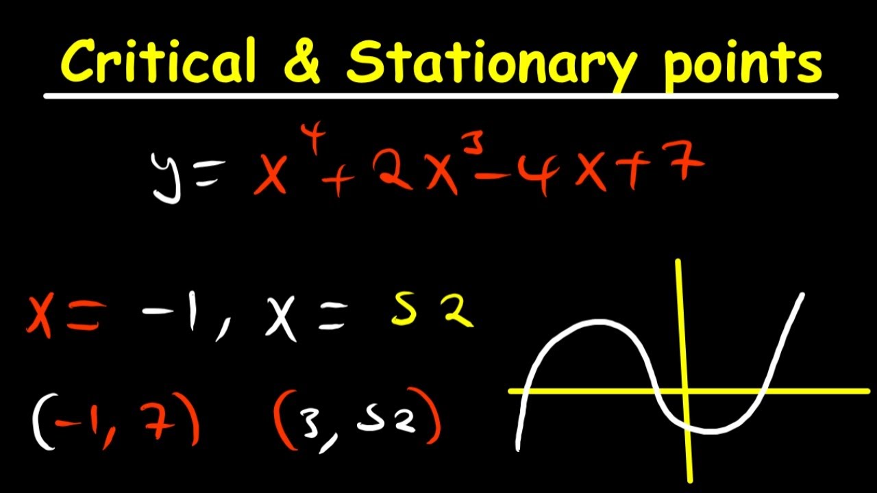
-The derivative is used to find the stationary points of the function, which are the points where the function's rate of change is zero.
What is a stationary point in the context of this script?
-A stationary point is a point on the graph of the function where the first derivative is zero, indicating a local maximum, minimum, or point of inflection.
How does the instructor find the x-values for the stationary points?
-The instructor finds the x-values for the stationary points by setting the first derivative of the function equal to zero and solving for x.
What is the importance of the leading coefficient in determining the end behavior of a cubic function?
-The leading coefficient determines whether the cubic function will rise or fall as x approaches positive or negative infinity. A positive leading coefficient means the function will rise to positive infinity as x increases.
How does the instructor use the second derivative to further analyze the cubic function?
-The script does not explicitly mention the use of the second derivative. However, typically, the second derivative can be used to determine the concavity of the function and further analyze the nature of the stationary points.
What is the final step the instructor asks the viewers to do?
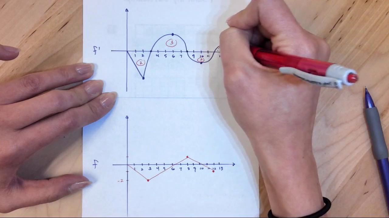
-The final step the instructor asks the viewers to do is to draw the function, its first derivative, and possibly the second derivative on a set of axes to compare their geometric features.
Outlines
📚 Introduction to Factorizing a Cubic Function
The first paragraph introduces the concept of factorizing a cubic function without the need for calculus. The speaker begins by factorizing a simple cubic function, taking a factor of x out and leaving a quadratic that is a perfect square. This allows the speaker to predict the shape of the function and its roots. The speaker also discusses the importance of the leading coefficient, which is positive in this case, indicating the function will grow large for large positive x values. Additionally, the speaker touches on the concept of stationary points and how they can be found using derivatives.
📈 Sketching the Function and Finding Stationary Points
The second paragraph focuses on sketching the cubic function and determining its stationary points geometrically. The speaker emphasizes the importance of drawing the function on a set of axes, with the first derivative and second derivative to be considered later. The speaker identifies the x-intercepts and stationary points, noting that one of the stationary points coincides with a root of the function. By substituting x-values into the function, the speaker finds the y-coordinates for the stationary points, which allows for a more accurate sketch of the function. The speaker also uses a horizontal line as a guide to ensure the function behaves as expected when plotted.
Mindmap
Keywords
💡Cubic Function
💡Factorization
💡Roots
💡Stationary Points
💡Derivative
💡Perfect Square
💡Graphing
💡Leading Coefficient
💡Y-Intercept
💡X-Intercept
💡Second Derivative
Highlights
Introduction to a simple cubic function for investigation without calculus.
Factorization of the cubic function to understand its roots and behavior.
Identification of a perfect square within the factorized quadratic.
Graphical representation of the cubic function with three roots.
Understanding the leading coefficient's impact on the function's end behavior.
Differentiation of the cubic function to find stationary points.
Derivative's role in revealing more about the function's geometry.
Finding the x-values for stationary points using the first derivative.
Clarification on the difference between zeros and intercepts of a function.
Graphical placement of stationary points based on the first derivative.
Misunderstanding about the symmetry of cubic functions compared to parabolas.
Calculation of the y-coordinate for the stationary point at x=1.
Plotting the function with known intercepts and stationary points.
Importance of accurate plotting for understanding function behavior.
Use of horizontal lines as guides for stationary points in graphing.
Emphasis on the final graphical result rather than the working process.
Instruction to draw three sets of axes for comparing function, first, and second derivatives.
Transcripts

5.0 / 5 (0 votes)
Thanks for rating: