Finding Stationary Points and Determining their Nature
TLDRThis educational script introduces the concept of stationary points in calculus, focusing on their identification and nature. It explains that stationary points occur where a function's graph changes direction, often marked by horizontal tangent lines. The script demonstrates how to find these points by setting the first derivative of a function to zero, using a cubic function as an example. It then describes two methods to determine the nature of stationary points: constructing a nature table to visualize the graph's behavior or using the second derivative test. The summary also touches on how to deduce where a function is increasing or decreasing from the stationary points, making it an essential guide for students tackling calculus.
Takeaways
- 📚 Stationary points are points on the graph of a function where the graph changes direction, indicated by horizontal tangent lines.
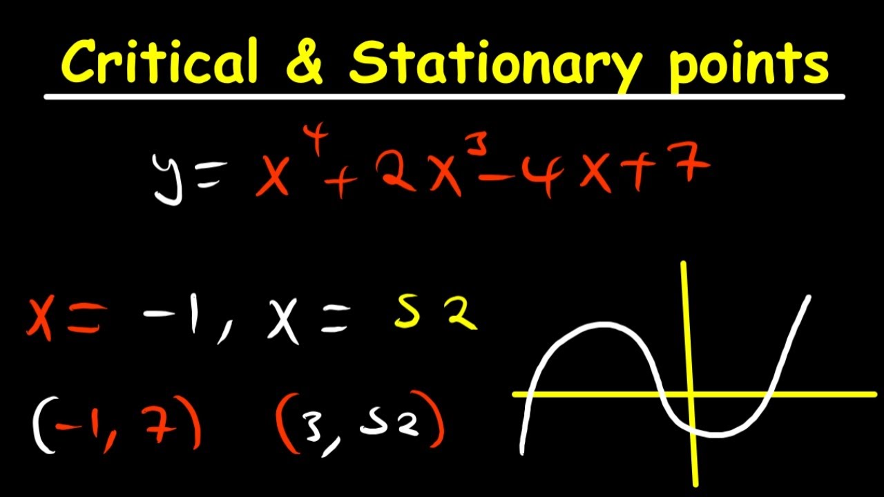
- 🔍 To find stationary points, one must take the derivative of the function and set it equal to zero, solving for the x-values where this occurs.
- 📈 The derivative, or the gradient, being zero at a point indicates a stationary point, as it represents a horizontal tangent line.
- 📝 For cubic functions, the derivative will be a quadratic function, and solving the resulting quadratic equation will give the x-coordinates of potential stationary points.
- 🧩 To determine the full coordinates of stationary points, substitute the x-values back into the original function to find the corresponding y-values.
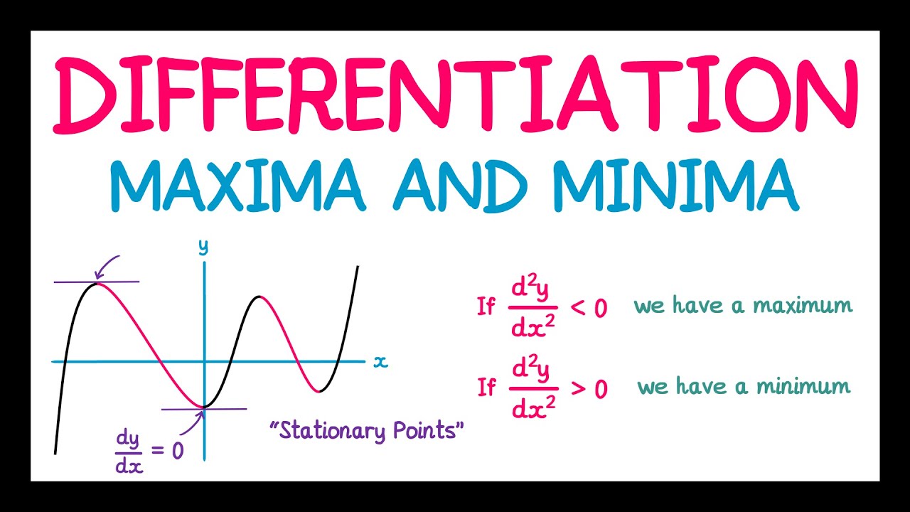
- 📊 There are three types of stationary points: maximum turning points, minimum turning points, and points of inflection, which require further analysis to identify.
- 📋 A nature table, which is a simplified sketch of the function's graph, can be used to determine the nature of stationary points by observing the sign of the derivative around these points.
- 🔢 The second derivative test involves taking the derivative of the first derivative and evaluating it at the stationary points; a positive second derivative indicates a minimum, while a negative one indicates a maximum.
- 📉 The nature table also provides information on where the function is increasing or decreasing, which is useful for understanding the function's behavior around stationary points.
- 📚 Understanding stationary points is crucial for calculus as it's a common topic that can yield significant marks with practice and procedural techniques.
Q & A
What are stationary points in the context of a function's graph?
-Stationary points are the points on the graph of a function where the graph changes direction, such as where it goes from increasing to decreasing or vice versa.
How can you determine the nature of a stationary point?
-The nature of a stationary point can be determined by using a nature table or by calculating the second derivative of the function. A positive second derivative indicates a minimum turning point, while a negative second derivative indicates a maximum turning point.
What is the relationship between the derivative of a function and its stationary points?
-At the stationary points, the derivative (or gradient) of the function is zero. This is because the tangent line to the graph at these points is horizontal.
How does the power rule apply to finding the derivative of a polynomial function?
-The power rule states that the derivative of a term ax^n is n*ax^(n-1). For a polynomial function, you apply the power rule to each term to find the derivative.
What is the expected number of solutions for the derivative of a cubic function?
-The derivative of a cubic function is a quadratic equation, which typically has two solutions. These solutions correspond to the x-coordinates of the stationary points of the original cubic function.
How can you find the full coordinates of a stationary point?
-To find the full coordinates of a stationary point, you substitute the x-coordinate(s) of the stationary point(s) back into the original function to find the corresponding y-coordinate(s).
What is a point of inflection and how does it differ from a maximum or minimum turning point?
-A point of inflection is a type of stationary point where the graph changes concavity but not monotonicity. It differs from a maximum or minimum turning point in that the graph does not have a pronounced peak or trough at these points.
How does the nature table help in understanding the behavior of a function around its stationary points?
-The nature table provides a mini sketch of the graph, showing whether the function is increasing or decreasing to the left and right of each stationary point. This helps in identifying the type of stationary point and the overall behavior of the function.
What is the significance of the second derivative test in determining the nature of a stationary point?
-The second derivative test provides a mathematical way to determine the nature of a stationary point without having to visualize the graph. It is particularly useful when the nature table is not conclusive or when a quick mathematical check is needed.
How can the information from the nature table be used to describe the intervals where the function is increasing or decreasing?
-The nature table can be used to identify the intervals where the function is increasing or decreasing by observing the sign of the derivative (or slope) at points around the stationary points. If the derivative is positive, the function is increasing; if negative, it is decreasing.
What is the importance of understanding stationary points in calculus?
-Understanding stationary points is crucial in calculus as they represent the local maxima, minima, or points of inflection of a function. These points are essential for analyzing the behavior of the function, optimizing problems, and understanding the shape of the graph.
Outlines
📚 Introduction to Stationary Points
This paragraph introduces the concept of stationary points, explaining that they are points on the graph of a function where the graph changes direction. The instructor uses a cubic function as an example, illustrating how stationary points can be identified by the slope of the tangent lines at those points. The key takeaway is that at stationary points, the derivative (or gradient) of the function equals zero. The process of finding stationary points involves taking the derivative of the function, setting it to zero, and solving for the variable, which in this case involves a polynomial function differentiated using the power rule.
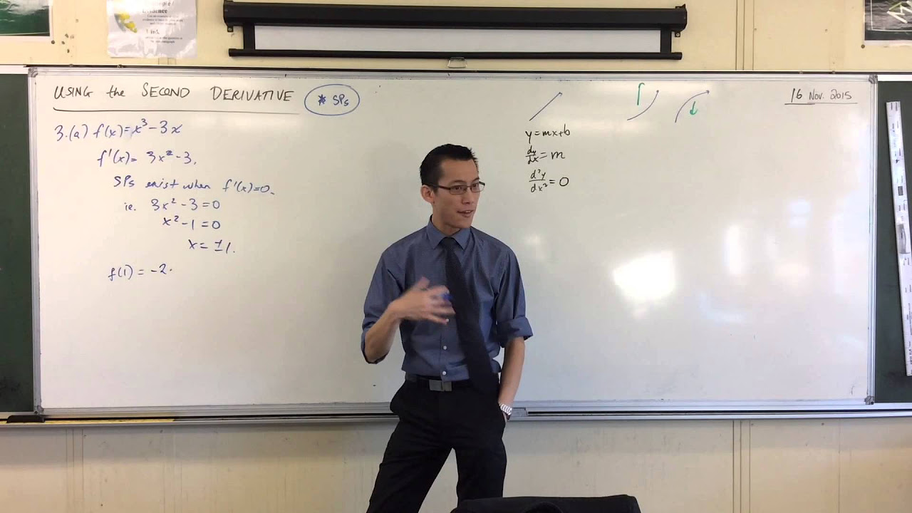
🔍 Locating Stationary Points Algebraically
The second paragraph delves into the algebraic process of finding stationary points. It explains that after differentiating a cubic function, a quadratic equation is obtained, which typically yields two solutions corresponding to the x-coordinates of the stationary points. The instructor demonstrates how to solve for these x-coordinates by factorizing the derivative set to zero. The solutions, x equals 0 and x equals 2, are then substituted back into the original function to find the corresponding y-coordinates, resulting in the full coordinates of the stationary points (0,0) and (2,4).
📈 Determining the Nature of Stationary Points
This paragraph discusses how to determine the nature of stationary points, which can be maximum turning points, minimum turning points, or points of inflection. Two methods are presented: the nature table and the second derivative test. The nature table is a simplified sketch of the graph that helps visualize the direction of the graph around the stationary points. By choosing test points and evaluating the sign of the derivative at these points, one can infer whether the graph is increasing or decreasing, thus identifying the nature of the stationary points. The second derivative test involves taking the derivative of the first derivative and evaluating it at the stationary points. A positive second derivative indicates a minimum turning point, while a negative one indicates a maximum. This paragraph also touches on the implications of stationary points for the overall shape of the graph and how they can be used to sketch the graph.
📘 Utilizing the Nature Table and Second Derivative for Analysis
The final paragraph emphasizes the utility of the nature table and the second derivative in analyzing the behavior of a function around its stationary points. It reiterates the process of filling out the nature table with test points and how this can reveal whether the function is increasing or decreasing in different intervals. The second derivative is also used to confirm the nature of the stationary points, with positive values indicating a minimum and negative values indicating a maximum. The paragraph concludes by highlighting the importance of understanding stationary points in calculus, noting that they are a common and valuable topic for exams due to their procedural nature and the potential to earn significant marks with practice.
Mindmap
Keywords
💡Stationary Points
💡Derivative
💡Graph
💡Cubic Function
💡Gradient
💡Nature Table
💡Second Derivative
💡Turning Point
💡Quadratic Equation
💡Increasing and Decreasing Functions
Highlights
Stationary points are points on the graph of a function where the graph changes direction.
Stationary points can be found by taking the derivative of a function and setting it to zero.
The derivative and gradient are the same concept, used to determine the slope of the tangent line at a point on the graph.
At stationary points, the derivative (or gradient) of the function is zero.
Differentiation is key to finding stationary points by setting the derivative equal to zero.
The process of finding stationary points involves algebraic manipulation without needing the graph's appearance.
For a cubic function, the derivative will be a quadratic function, suggesting two potential stationary points.
Solving the equation set by the derivative equal to zero gives the x-coordinates of stationary points.
The y-coordinates of stationary points are found by substituting the x-coordinates back into the original function.
Stationary points can be classified as maximum turning points, minimum turning points, or points of inflection.
A nature table or second derivative test can be used to determine the nature of stationary points.
A nature table is a simplified sketch of the graph that helps in identifying the type of stationary point.
The second derivative test involves taking the derivative of the first derivative and evaluating it at stationary points.
A positive second derivative at a stationary point indicates a minimum turning point, while a negative indicates a maximum.
If the second derivative is zero at a stationary point, the test is inconclusive and a nature table should be used.
A nature table not only helps in identifying stationary points but also in determining where the function is increasing or decreasing.
Understanding stationary points is crucial for sketching graphs and is a common topic in calculus with significant marks.
Transcripts
Browse More Related Video


5.0 / 5 (0 votes)
Thanks for rating: