Finding the Area Under the ROC Curve — Topic 91 of Machine Learning Foundations
TLDRThe video script outlines a practical demonstration of calculating the area under the Receiver Operating Characteristic (ROC) curve using Python code. It emphasizes the significance of the ROC curve as a comprehensive metric for evaluating binary classification models in machine learning. The demonstration employs the trapezoidal rule through the `auc` method from the scikit-learn library, utilizing five given coordinate points to approximate the area under the curve. The result, an area of 0.75, is visually confirmed against a chart provided in the video. This exercise concludes the calculus content in the speaker's machine learning foundation series, with a promise of a summary video and recommended resources for further exploration into calculus.
Takeaways
- 📈 The video demonstrates how to calculate the area under the Receiver Operating Characteristic (ROC) curve using Python code.
- 🧮 The ROC curve is a powerful metric used in machine learning to evaluate the quality of a binary classification model.
- 📊 The area under the ROC curve is calculated using integral calculus, specifically the trapezoidal rule, which is a numerical approach.
- 📚 The scikit-learn library's `metrics` module provides an `auc` method that can be used to find the area under the curve.
- 📍 Five specific coordinates (0,0), (0,0.5), (0.5,0.5), (0.5,1), and (1,1) are used to represent the ROC curve for the calculation.
- 💻 The video is a part of a machine learning foundation series focusing on integration and its application in machine learning.
- 🔗 The method uses numerical integration to approximate the area under the curve when an explicit function is not available.
- 📝 The coordinates are input into the `auc` method as two vectors of x and y values to calculate the area.
- 🔢 The calculated area under the curve in the example is 0.75, which can be visually confirmed by the chart provided.
- 🔍 The video concludes with a suggestion to look at the chart to verify the calculated area and understand the concept better.
- 🚀 The next video in the series will summarize the calculus content covered and provide resources for further learning.
Q & A
What is the purpose of the video?
-The video demonstrates how to calculate the area under the Receiver Operating Characteristic (ROC) curve using Python code, which is a machine learning specific application of integral calculus.
What is the Receiver Operating Characteristic (ROC) curve?
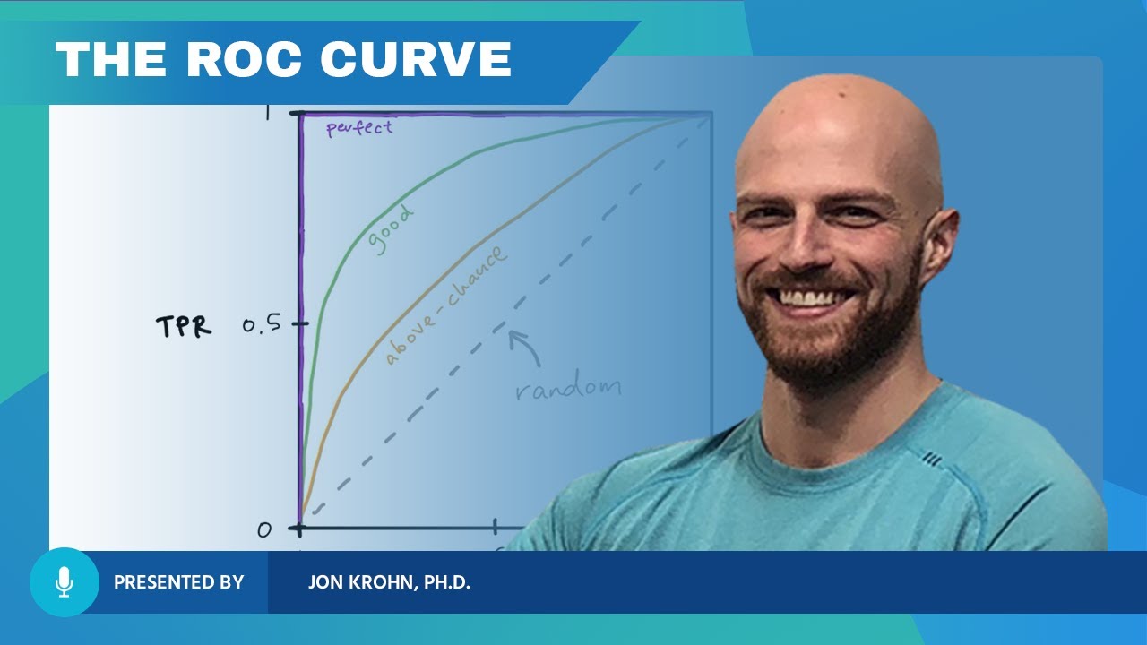
-The ROC curve is a graphical representation that allows for the assessment of the quality of a binary classification model by plotting the true positive rate against the false positive rate at various threshold settings.
How does the video use integral calculus to find the area under the ROC curve?
-The video uses the numerical approach of the trapezoidal rule from the scikit-learn metrics module to calculate the area under the curve.
What is the numerical method used to calculate the area under the curve?
-The trapezoidal rule is used, which is a numerical integration technique that approximates the area under a curve as a series of trapezoids.
How many coordinates are used in the video to calculate the area under the ROC curve?
-Five coordinates are used to calculate the area under the ROC curve.
What are the five coordinates used in the video?
-The five coordinates are (0,0), (0,0.5), (0.5,0.5), (0.5,1), and (1,1).
How does the video approach the problem of not having a function to calculate the area under the curve?
-The video uses the available xy-coordinates and the auc method from the scikit-learn metrics module to numerically calculate the area under the curve.
What is the area under the ROC curve calculated in the video?
-The area under the ROC curve calculated in the video is 0.75.
How can the calculated area under the ROC curve be visually confirmed?
-The calculated area can be visually confirmed by looking at the chart provided in the video, where three quarters of the area under the ROC curve is filled in.
What is the next step after the calculus content in the machine learning foundation series?
-The next step is a quick summary of everything covered in the series, followed by a list of the presenter's favorite resources for further study into calculus topics.
Why is the ROC curve considered a nuanced and powerful metric?
-The ROC curve is considered nuanced and powerful because it provides a single summary metric that encapsulates the trade-off between the true positive rate and the false positive rate, offering a comprehensive view of a classification model's performance.
What is the significance of the area under the ROC curve in machine learning?
-The area under the ROC curve is significant because it quantifies the overall ability of a classification model to distinguish between classes. An area of 1 indicates a perfect model, while an area of 0.5 suggests the model is no better than random guessing.
Outlines
📈 Calculating the Area Under the ROC Curve
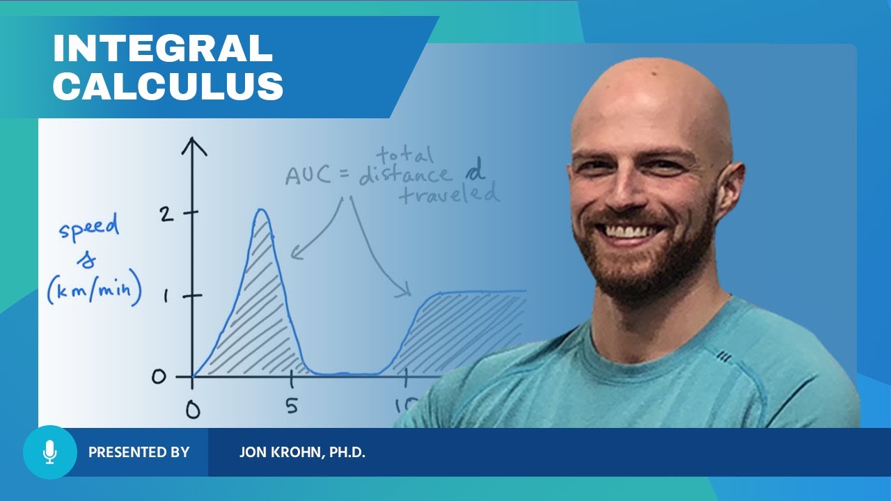
This paragraph introduces the application of integral calculus to machine learning by calculating the area under the Receiver Operating Characteristic (ROC) curve. The ROC curve is a powerful metric for assessing the quality of a binary classification model. The video demonstrates a hands-on, automated approach using Python code. It guides viewers to a specific section of a Jupyter notebook where the calculation takes place. The process involves using numerical integration, specifically the trapezoidal rule, to calculate the area under the curve from given coordinates. The scikit-learn library's 'auc' method is used for this purpose. The video concludes by confirming the calculated area of 0.75 visually against a chart and mentions a forthcoming summary of calculus content in the machine learning foundation series.
Mindmap
Keywords
💡Python code
💡Area under the curve (AUC)
💡Receiver Operating Characteristic (ROC)
💡Machine Learning
💡Integral Calculus
💡Trapezoidal Rule
💡Scikit-learn
💡Numerical Approach
💡Coordinates
💡Vectors
💡Colab Notebook
Highlights
The video demonstrates calculating the area under the Receiver Operating Characteristic (ROC) curve using Python code.
The ROC curve is a nuanced and powerful summary metric for assessing the quality of a binary classification model in machine learning.
The area under the ROC curve is calculated using integral calculus, specifically the trapezoidal rule.
The demonstration uses five specific coordinates to calculate the area under the curve.
The scikit-learn library's metrics module provides an 'auc' method for numerical integration.
The 'auc' method is applied to two vectors of x and y coordinates to find the area under the curve.
The result of the area under the curve is 0.75, which can be visually confirmed on the provided chart.
The video is part of a machine learning foundation series that covers integration in calculus.
The video provides a hands-on code demo for a quick and automated calculation of the area under the ROC curve.
The coordinates used in the demo are (0,0), (0,0.5), (0.5,0.5), (0.5,1), and (1,1).
The integration process involves creating vectors for x and y coordinates and using them in the 'auc' method.
The video concludes with a summary of the calculus content covered in the machine learning foundation series.
The next video in the series will provide a summary and resources for further study of calculus topics.
The numerical approach used in the demo is based on the trapezoidal rule, which can be explored further in the provided link.
The video assumes prior knowledge of the ROC curve from earlier segments in the series.
The integration is performed using a Jupyter notebook, which is a popular tool for data analysis and machine learning.
The video emphasizes the practical application of calculus in the context of machine learning model evaluation.
The hands-on demo shows how to run the Jupyter notebook and execute the necessary code cells.
The final section of the Jupyter notebook is dedicated to calculating the area under the ROC curve.
The video provides a clear, step-by-step guide on how to perform the calculation using Python and scikit-learn.
Transcripts
Browse More Related Video
The ROC Curve (Receiver-Operating Characteristic Curve) — Topic 84 of Machine Learning Foundations
ROC and AUC, Clearly Explained!
What Integral Calculus Is — Topic 85 of Machine Learning Foundations

ROC Curves

Calculus Applications – Topic 46 of Machine Learning Foundations

My Favorite Calculus Resources — Topic 92 of Machine Learning Foundations
5.0 / 5 (0 votes)
Thanks for rating: