The Line Equation as a Tensor Graph — Topic 65 of Machine Learning Foundations
TLDRThis video script outlines a machine learning tutorial that focuses on using automatic differentiation to fit a simple linear model to a set of data points. The process begins with representing the line equation y = mx + b as a directed acyclic graph (DAG), where nodes represent variables and operations. The script then guides viewers through setting up the computational graph in PyTorch, a popular machine learning library. The tutorial involves creating a synthetic dataset based on a line equation with added noise to simulate real-world data. Parameters for the line equation are initialized randomly, a common practice in machine learning to allow models to learn from the data. The script emphasizes the scalability of the approach to complex models with numerous parameters and data points. The video concludes with a teaser for the next part of the series, which will delve into machine learning theory and the application of automatic differentiation to fit the line to the data points.
Takeaways
- 📈 The video discusses setting up automatic differentiation within a machine learning loop by representing an equation as a tensor graph in PyTorch.
- 🔍 The simple line equation y = mx + b is used to demonstrate the process, where m is the slope and b is the y-intercept.
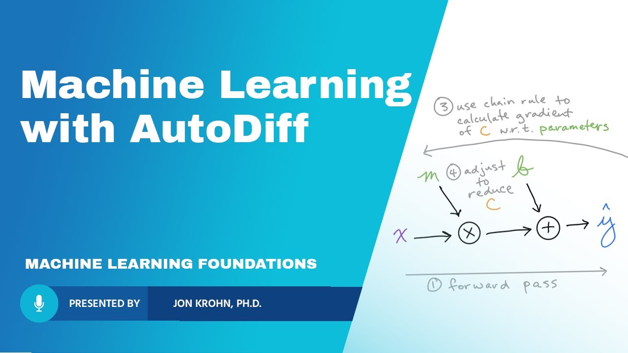
- 🌟 The line equation is represented as a Directed Acyclic Graph (DAG), which consists of nodes and directed edges with no cycles.
- 💻 A hands-on code demonstration is provided using the 'regression in PyTorch' notebook from a GitHub repository.
- 📊 Data points for the line equation are generated with a made-up example of a drug dosage for treating Alzheimer's disease, including random noise to simulate real-world sampling error.
- 🔧 PyTorch's automatic differentiation capabilities are utilized to fit a straight line to the data points, contrasting with algebraic or statistical approaches.
- 📉 The initial parameters for the line (m and b) are randomly initialized near-zero values, a common practice in machine learning to allow the model to learn the correct parameters.
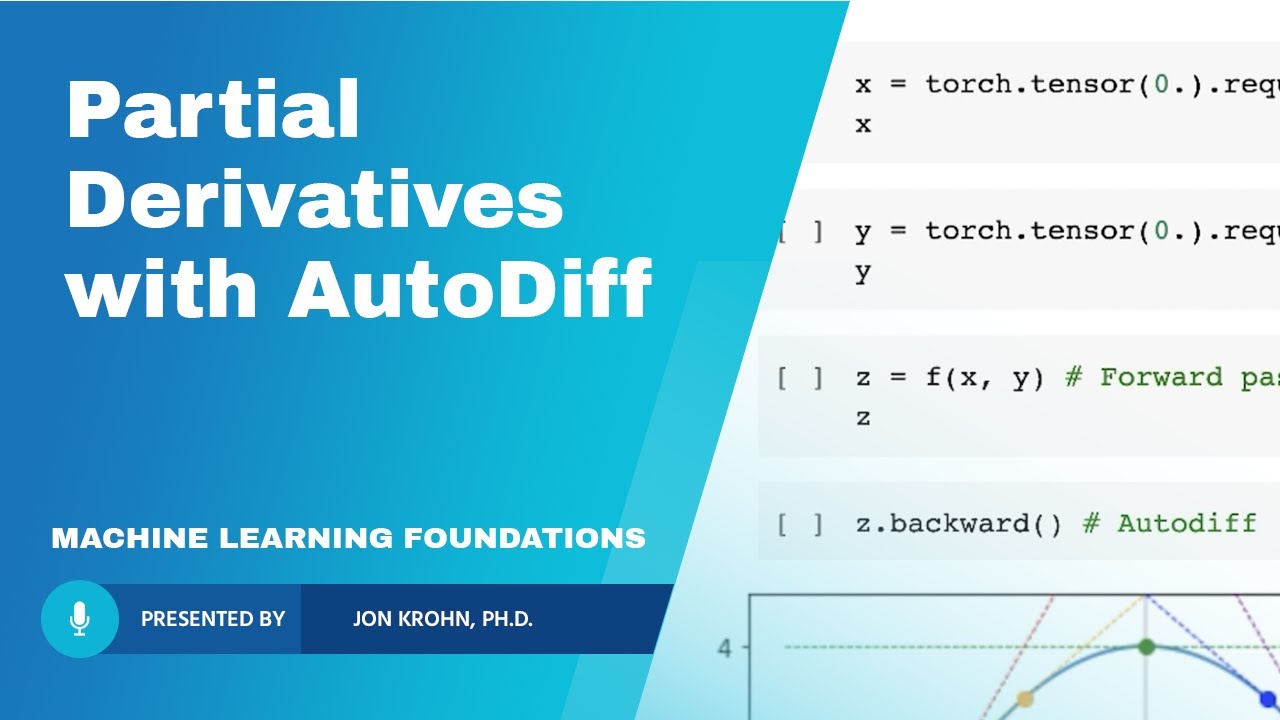
- 🔑 The 'requires_grad' method in PyTorch is used to track gradients, which is essential for performing differentiation and optimizing the line equation parameters.
- 📈 A regression plot function is introduced to visualize the relationship between the input (x) and output (y) variables, along with the line that the model is learning to fit.
- 🎯 The process scales to complex models with millions of parameters and data points, unlike some other methods that do not scale as effectively.
- ⏭ The next steps involve learning more machine learning theory and applying it to fit the line to the data points using the regression method in PyTorch.
Q & A
What is the purpose of representing an equation as a tensor graph in machine learning?
-Representing an equation as a tensor graph allows for the application of automatic differentiation within a machine learning loop. This is essential for training models by adjusting parameters to minimize the difference between predicted and actual outcomes.
What is a Directed Acyclic Graph (DAG)?
-A Directed Acyclic Graph (DAG) is a finite directed graph with no directed cycles. In the context of machine learning, it's used to represent the flow of information through a system, where each node represents an operation or a parameter, and edges represent the flow of data.
How is the line equation y = mx + b represented in a DAG?
-In a DAG, the line equation y = mx + b is represented with nodes for the input x, output y, and parameters m (slope) and b (y-intercept). Operations such as multiplication (m times x) and addition (adding b to the product) are also represented as nodes. Directed edges connect these nodes, representing the flow of data through the equation.
Why is it necessary to initialize model parameters with random near-zero values in machine learning?
-Initializing model parameters with random near-zero values is a common practice in machine learning that helps the model learn from the data without bias. It ensures that the learning process starts afresh and does not make assumptions based on the initial parameter values.
What role does PyTorch play in the automatic differentiation process?
-PyTorch is a machine learning library that provides tools for building and training neural networks. It plays a crucial role in the automatic differentiation process by tracking operations on tensors and computing gradients that are necessary for updating parameters during the training process.
How does adding random noise to the y values simulate real-world scenarios in the provided example?
-Adding random noise to the y values simulates the imperfect relationship between x and y variables that is often observed in real-world data. It introduces variability that a model must learn to account for, making the model more robust and better suited to handle real-world data.
What is the significance of the 'requires_grad' method in PyTorch?
-The 'requires_grad' method in PyTorch is used to specify whether the values contained in a tensor require the computation of gradients. This is important for tensors that are parameters of a model, as gradients are needed to update these parameters during training.
How does the machine learning approach to fitting a line scale with the size of the model and data?
-The machine learning approach to fitting a line, as demonstrated in the script, can scale to models with millions or even billions of parameters and data points. This is in contrast to other methods like linear algebra or statistics, which do not scale as effectively for large models and datasets.
What is the significance of the negative relationship between drug dosage and patient's forgetfulness in the Alzheimer's disease example?
-The negative relationship signifies that as the dosage of the hypothetical Alzheimer's drug increases, the level of forgetfulness in patients decreases. This is a common type of relationship in many real-world scenarios where increasing one variable leads to a decrease in another.
Why is it important to understand the underlying model parameters when creating y values in the script?
-Understanding the underlying model parameters is important because it allows for the creation of y values that accurately reflect the relationship defined by the line equation. This knowledge is crucial for training the model effectively, as it provides a benchmark against which the model's predictions can be compared and improved.
What are the steps involved in using the machine learning approach to fit a line to data points in PyTorch?
-The steps include: (1) Representing the line equation as a DAG, (2) Initializing the model parameters randomly, (3) Using PyTorch to track gradients and perform automatic differentiation, (4) Defining the computational graph with all components, (5) Applying machine learning theory to update parameters and fit the line to the data points.
Outlines
📈 Setting Up Automatic Differentiation for Machine Learning
The video begins by introducing the concept of automatic differentiation within a machine learning context. It discusses representing equations as tensor graphs, specifically using a simple linear equation (y = mx + b) as an example. The process involves creating a directed acyclic graph (DAG) with nodes for inputs, outputs, and parameters, as well as operations like multiplication and addition. The video also mentions the upcoming discussion on DAGs in the algorithms and data structures portion of the machine learning foundation series. The viewer is guided to a GitHub repository for hands-on coding with PyTorch to implement the DAG for the line equation.
🧮 Using Calculus for Linear Regression
The script moves on to applying calculus for linear regression by manually creating data points based on a line equation with an added noise component to simulate real-world data imperfections. The data points represent a hypothetical drug dosage for Alzheimer's treatment and its effect on patient forgetfulness. The video uses a scatter plot to visualize the relationship between the drug dosage and the outcome. The process involves importing necessary libraries, creating synthetic data, and plotting it. The script also touches on probability distributions and random processes, which will be covered in more depth in a later subject of the series.
🔧 Initializing Parameters for the Regression Model
The video explains the common machine learning practice of initializing model parameters with random near-zero values. This is crucial for models ranging from simple to complex, including deep learning models. The script justifies the use of a random value for the slope (m) and y-intercept (b) in the line equation, emphasizing the importance of not starting with values that are too close to the actual solution to demonstrate the model's learning process. The video also mentions the scalability of the machine learning approach being demonstrated, contrasting it with other methods like linear algebra or statistics that do not scale as effectively.
🎯 Gradient Tracking for Automatic Differentiation
The script details the process of setting up gradient tracking for automatic differentiation in PyTorch. This involves marking tensor variables as requiring gradients, which allows the model to track the gradient flow from the outcome back to the parameters. The video demonstrates initializing the y-intercept parameter (b) with a near-zero value and creating a regression plot function to visualize the data points and the line that the model is learning to fit. The function takes the current parameters and plots the line, showing the initial fit before the machine learning process begins.
🔄 Linking Components for Model Training
The final paragraph outlines the preparation for linking all components of the computational graph, including the initialized parameters and the data points. The script discusses the creation of a regression method that combines the parameters and inputs to generate the output. The video concludes with a teaser for the next part of the series, which will cover more machine learning theory before returning to the PyTorch notebook to fit the line to the data points using the theory. The presenter also encourages viewers to subscribe, engage with the content, and follow on social media for updates.
📢 Stay Connected for Future Content
The video script concludes with a brief invitation for viewers to connect with the presenter on social media platforms, specifically mentioning LinkedIn and Twitter. This is a standard practice to build a community and engage with the audience beyond the video content.
Mindmap
Keywords
💡Automatic Differentiation
💡Tensor Graph
💡Directed Acyclic Graph (DAG)
💡Machine Learning Model
💡Linear Regression
💡Slope (m)
💡Y-Intercept (b)
💡Random Initialization
💡Gradient
💡PyTorch
💡Colab
Highlights
The video introduces automatic differentiation within a machine learning loop by representing an equation as a tensor graph.
A simple linear equation y = mx + b is used to demonstrate the concept, where m is the slope and b is the y-intercept.
The equation is represented as a Directed Acyclic Graph (DAG), consisting of nodes and directed edges with no cycles.
Nodes in the graph include an input node (x), output node (y), and parameters (m and b) shown in green.
Operations such as multiplication (m times x) and addition (adding b to the product) act as nodes within the graph.
Tensors hold information about the nodes, with directed edges representing the flow of information.
The video provides a hands-on code demonstration using PyTorch to create the DAG for the simple line equation.
The regression in PyTorch notebook is used, which is part of a machine learning foundations series on GitHub.
The notebook utilizes automatic differentiation in PyTorch to fit a straight line to data points.
Data points are generated using a made-up example of a drug dosage for treating Alzheimer's disease.
Random normally distributed noise is added to simulate sampling error and account for real-world imperfect relationships.
The model parameters are initialized with random near-zero values, a common practice in machine learning.
The video explains the importance of not initializing parameters too close to the true values to allow the model to learn.
The `requires_grad` method in PyTorch is used to track gradients, enabling automatic differentiation.
A regression plot function is created to visualize the relationship between x and y and the line fitting process.
The video emphasizes that the machine learning approach demonstrated scales to models with millions of parameters and data points.
The next steps involve learning more machine learning theory and applying it to fit the line to the data points using PyTorch.
The video concludes with an invitation to subscribe for the next tutorial in the series and engage with the content through likes, comments, and social media.
Transcripts
Browse More Related Video
Machine Learning from First Principles, with PyTorch AutoDiff — Topic 66 of ML Foundations
Calculating Partial Derivatives with PyTorch AutoDiff — Topic 69 of Machine Learning Foundations

The Gradient of Mean Squared Error — Topic 78 of Machine Learning Foundations

Interpreting Graphs in Chemistry

Calculus Chapter 2 Lecture 14 BONUS

Build A Machine Learning Web App From Scratch
5.0 / 5 (0 votes)
Thanks for rating: