Calculating Power and the Probability of a Type II Error (A One-Tailed Example)
TLDRThe video script presents a detailed explanation of calculating statistical power and the probability of a Type II error, often denoted as beta, using a one-sample Z test as an example. It begins by establishing the scenario of sampling from a normally distributed population with a known standard deviation and an unknown mean. The null hypothesis is set to test if the population mean is 50 against a one-sided alternative hypothesis, with a significance level of 0.09. The script explains how to determine the rejection region for the null hypothesis based on the Z test statistic and the sample mean. It then explores the probability of committing a Type II error when the true mean is 43 and calculates the statistical power when the true mean is 40. The process involves visualizing the sampling distribution of the sample mean, standardizing the test statistic, and using the standard normal curve to find the corresponding probabilities. The video concludes by emphasizing the importance of correctly identifying the required areas for power calculations, regardless of the alternative hypothesis.
Takeaways
- 📊 **Z Test for Mean**: The example discusses a one-sample Z test used to test the null hypothesis about a population mean when the population standard deviation is known.
- 🎯 **Null Hypothesis**: The null hypothesis (H0) is that the population mean (μ) is 50, and it's being tested against a one-sided alternative hypothesis that μ is less than 50.
- 🔍 **Significance Level (α)**: A significance level of 0.09 is chosen, meaning there's a 9% chance of committing a type I error if the null hypothesis is true.
- 📉 **Rejection Region**: The null hypothesis will be rejected if the Z statistic is less than or equal to -1.34, which corresponds to the left tail of the standard normal distribution at α = 0.09.
- 🔢 **Sample Mean Rejection**: The sample mean (X̄) will lead to the rejection of the null hypothesis if it's less than or equal to 45.31, derived from the Z statistic.
- 🚫 **Type I Error**: The probability of a type I error is the given α level, which is the probability of rejecting a true null hypothesis.
- 🛑 **Type II Error (β)**: The probability of a type II error is the likelihood of not rejecting a false null hypothesis when the true mean is 43, calculated as β ≈ 0.255.
- ✅ **Power of Test**: The power of the test is 1 - β, which is the probability of correctly rejecting a false null hypothesis. In this case, it's approximately 0.745 when the true mean is 43.
- 📈 **Increased Power**: If the true mean is further from the hypothesized mean (e.g., μ = 40), the power of the test increases, making it more likely to correctly reject the null hypothesis.
- 📐 **Standardization**: The calculation of type II error and test power involves standardizing the sample mean to a Z score for comparison against the rejection region.
- 📋 **Visual Aids**: The script uses visual aids such as plotting the standard normal curve and shading areas to represent the probabilities of type I and type II errors and the power of the test.
Q & A
What is the significance level (alpha) chosen for the one-sample Z test in the example?
-The significance level (alpha) chosen for the test is 0.09.
What is the known population standard deviation (sigma) in the example?
-The known population standard deviation (sigma) is 21.
What is the null hypothesis being tested in the example?
-The null hypothesis being tested is that the population mean (mu) is 50.
What is the Z value that corresponds to the chosen alpha level of 0.09?
-The Z value that corresponds to the alpha level of 0.09 is -1.34.
How is the rejection region in terms of the sample mean (X bar) calculated?
-The rejection region in terms of the sample mean (X bar) is calculated as 50 plus (21 / √36) times -1.34, which equals 45.31.
What is the probability of committing a type I error in this scenario?
-The probability of committing a type I error, which is the same as the given alpha level, is 0.09.
If the true population mean is 43, what is the probability of committing a type II error?
-The probability of committing a type II error when the true population mean is 43 is approximately 0.255.
What is the power of the test and how is it calculated?
-The power of the test is the probability of rejecting the null hypothesis when it is false, which is calculated as 1 minus the probability of a type II error (1 - beta).
If the true population mean is 40, what is the power of the test?
-If the true population mean is 40, the power of the test is the probability that the sample mean (X bar) is less than or equal to 45.31. This corresponds to an area to the left of 1.517 on the standard normal curve, which is approximately 0.935.
How does the sampling distribution of the sample mean (X bar) change if the true population mean is different from the hypothesized mean?
-The sampling distribution of the sample mean (X bar) will be centered around the true population mean. If the true mean is different from the hypothesized mean, the distribution will be shifted accordingly, affecting the probabilities associated with type I and type II errors.
What is the relationship between the sample size (n) and the standard deviation of the sample mean (sigma/√n)?
-The standard deviation of the sample mean (sigma/√n) decreases as the sample size (n) increases, which means that larger sample sizes result in a more precise estimate of the population mean.
How do the concepts of type I and type II errors relate to the significance level (alpha) and the power of the test?
-The significance level (alpha) determines the probability of a type I error, which is the chance of rejecting a true null hypothesis. The power of the test, which is the probability of correctly rejecting a false null hypothesis, is influenced by the alpha level, the true state of nature (the actual value of the population mean), and the sample size.
Outlines
🔍 Calculating Power and Type II Error Probability
This paragraph discusses the process of calculating statistical power and the probability of a type II error, also known as beta, within the context of a one-sample Z test on a mean. It explains that with a known population standard deviation (sigma = 21) and an unknown population mean (mu), we aim to test if the population mean is 50 against a one-sided alternative hypothesis with a significance level of 0.09. The Z test statistic is used for this normally distributed population. The rejection region for the null hypothesis is determined by the Z value corresponding to an area of 0.09 to the left in the standard normal distribution, which is -1.34. The sample mean (X bar) rejection region is then calculated to be less than or equal to 45.31. The paragraph also explores the probability of a type II error when the true population mean is 43, which is the probability of not rejecting the null hypothesis when it is false, by comparing the sample mean distributions under the null hypothesis and the alternative scenario where mu is 43.
📊 Visualizing Type II Error and Test Power
The second paragraph delves into visualizing the type II error and calculating the test's power. It describes the scenario where the true population mean is 43, and the null hypothesis that mu is 50 is false. The probability of a type II error is the probability of not rejecting the null hypothesis when the sample mean (X bar) is greater than 45.31. This is visually represented by shading the area to the right of 45.31 on the distribution curve. The paragraph then standardizes the calculation by expressing X bar as a Z score, leading to the probability that Z is greater than 0.66, which is found to be approximately 0.255. The test power, which is the probability of correctly rejecting a false null hypothesis, is then calculated as 1-beta, resulting in 0.745. The paragraph further illustrates another power calculation example where the true mean is 40, showing the visual representation of the sampling distribution and the calculation of power as the probability that the sample mean is less than or equal to 45.31.
🧮 Standardizing for Power Calculations
The final paragraph focuses on the standardization process for power calculations under alternative hypotheses. It explains that the same logic used for calculating power when mu is less than the hypothesized value can be applied to other scenarios, such as when mu is greater or not equal to the hypothesized value. However, the specific areas under the standard normal curve that are considered will change. The paragraph emphasizes the importance of carefully considering the correct areas for power calculations. It concludes with a reminder to use the standard normal curve to find the area to the left of the Z value, which in the provided example is 1.517, corresponding to a power of approximately 0.935.
Mindmap
Keywords
💡Power of a test
💡Type II error
💡Null hypothesis
💡Alternative hypothesis
💡Significance level (alpha)
💡Z test statistic
💡Population mean (mu)
💡Population standard deviation (sigma)
💡Sample mean (X bar)
💡Rejection region
💡Sampling distribution
Highlights
Calculating power and the probability of a type II error, often referred to as beta, is demonstrated using a one-sample Z test on a mean.
The population standard deviation sigma is known to be 21, while the population mean mu is unknown.
The null hypothesis is that the population mean is 50, and a one-sided alternative hypothesis is being tested.
A significance level of 0.09 is chosen for the test, which is a measure of the probability of a type I error.
The Z test statistic is used for the hypothesis test, assuming a standard normal distribution under the null hypothesis.
The rejection region for the null hypothesis is determined by finding the Z value corresponding to an area of 0.09 to the left, which is -1.34.
The sample mean rejection region is reexpressed as X bar less than or equal to 45.31, derived from the Z test statistic.
The probability of committing a type I error, or rejecting the true null hypothesis, is the given alpha level of 0.09.
The probability of a type II error is calculated when the true population mean is 43, which is the probability of not rejecting the null hypothesis when it is false.
The type II error probability is found by calculating the area to the right of the rejection region under the assumption that mu is 43.
The sampling distributions of X bar under the null hypothesis and the alternative scenario where mu is 43 are visually represented for comparison.
The probability of a type II error when mu is 43 is approximately 0.255, found by standardizing the sample mean to a Z score.
The power of the test, or the probability of correctly rejecting a false null hypothesis, is calculated as 1-beta, which is 1-0.255 or 0.745.
Another power calculation example is given where the true population mean is 40, showing how to find the test's power in different scenarios.
The power is visualized by shading the area under the sampling distribution of X bar that corresponds to rejecting the null hypothesis when mu is 40.
The power of the test in the scenario where mu is 40 is approximately 0.935, indicating a high likelihood of correctly rejecting the null hypothesis.
The process of power calculation under different alternative hypotheses is emphasized, noting that while the logic remains the same, the required areas for calculation will differ.
The importance of correctly identifying the areas for power calculations is stressed to ensure accurate results in hypothesis testing.
Transcripts
Browse More Related Video
Introduction to Type I and Type II errors | AP Statistics | Khan Academy
Hypothesis Testing Explained | Statistics Tutorial | MarinStatsLectures
8.3.2 Testing a Claim About a Mean - Sigma Known and When the Sampling Distribution Isn't Normal
Type 1 errors | Inferential statistics | Probability and Statistics | Khan Academy
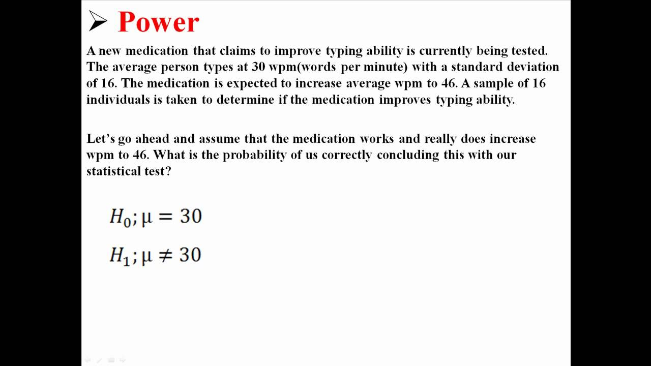
Power
Hypothesis Testing: Calculations and Interpretations| Statistics Tutorial #13 | MarinStatsLectures
5.0 / 5 (0 votes)
Thanks for rating: