Autonomous Equations, Equilibrium Solutions, and Stability
TLDRThe video script delves into the concept of autonomous differential equations, which are a type of first-order differential equation where the derivative of the dependent variable y is solely a function of y, with no explicit dependence on the independent variable t. The presenter illustrates the characteristics of these equations using the example ( dy/dt = 1 + y(1 - y) ). Key points include identifying equilibrium points where the derivative equals zero, such as y = -1 and y = 1, and discussing the stability of these points. The script explains that an equilibrium point is asymptotically stable if nearby solutions tend to converge to it over time, whereas it is unstable if nearby solutions diverge. The use of GeoGebra to plot slope fields visually demonstrates the behavior of solutions and their approach to equilibrium points. The video serves as an introduction to the topic, inviting viewers to explore further through comments and subsequent videos.
Takeaways
- 📘 Autonomous differential equations are a type of first-order differential equation where the derivative only depends explicitly on the dependent variable y, not on the independent variable t.
- 🔍 To find when the derivative is zero in an autonomous equation, solve for y when the right-hand side of the equation equals zero, which gives critical points.
- 📊 Use computer software like GeoGebra to plot slope fields, which can help visualize the behavior of solutions to autonomous differential equations.
- 🎯 Equilibrium solutions occur when y equals a constant value that makes the derivative zero; these points are where the slope field is horizontal.
- 🔄 Above and below the equilibrium points, the slope field indicates whether the equilibrium is stable (slopes tend towards the point) or unstable (slopes tend away from the point).
- 🔺 An equilibrium point y = a is asymptotically stable if solutions starting near a tend towards a as time goes to infinity.
- ⛔ An equilibrium point y = a is unstable if solutions starting near a tend to move away from a as time progresses.
- 🔀 The behavior of the slope field between equilibrium points can indicate the general trend of solutions, such as moving towards one equilibrium point or another.
- 📈 For y > 1, the slope is negative, indicating that values of y will decrease towards the equilibrium point, showing stability.
- 📉 For y < -1, the slope is also negative, but it indicates that solutions starting near this unstable equilibrium point will move away, towards negative infinity.
- ➿ The value of y = 0 serves as an example where the slope is positive, indicating an upward trend towards the stable equilibrium point y = 1.
- ✍️ The definitions and properties of autonomous equations and their equilibrium points are crucial for understanding the long-term behavior of solutions.
Q & A
What is an autonomous differential equation?
-An autonomous differential equation is a type of first-order differential equation where the derivative only depends explicitly on the dependent variable y, and not on the independent variable t.
What are the critical points in the context of differential equations?
-Critical points in differential equations are the points where the derivative is equal to zero. They often represent equilibrium or steady states of a system.
How does the behavior of the slope field around the equilibrium points help determine the stability of the equilibrium solutions?
-The behavior of the slope field around the equilibrium points indicates whether the solutions tend towards or away from these points. If the slope is negative above and positive below an equilibrium point, it is stable (asymptotically stable). If the slope is negative above and below, the equilibrium is unstable.
What is the significance of the equilibrium point y = 1 in the given example?
-In the example provided, y = 1 is an asymptotically stable equilibrium point. This means that if the system starts near y = 1, it will tend towards this value as time goes to infinity.
How does the equilibrium point y = -1 differ from y = 1 in terms of stability?
-The equilibrium point y = -1 is an unstable equilibrium point. Solutions that start near y = -1 tend to move away from this point, either towards positive infinity or negative infinity, rather than converging to it.
What is the role of the independent variable t in an autonomous differential equation?
-In an autonomous differential equation, the independent variable t does not appear explicitly in the equation. The derivative is a function solely of the dependent variable y, which still depends on t, but t's role is implicit rather than explicit.
How does the concept of equilibrium solutions apply to real-world systems?
-Equilibrium solutions are used to model steady states in real-world systems. For example, in physics, they can represent a state where forces balance out, or in biology, they can indicate a stable population size.
What is the importance of understanding the stability of equilibrium points in differential equations?
-Understanding the stability of equilibrium points is crucial as it helps predict the long-term behavior of a system. It can inform decisions in control theory, engineering, economics, and other fields where stability is a key concern.
What is the role of a computer in graphing slope fields for autonomous differential equations?
-A computer can help visualize the slope field by plotting the direction of the slope (the derivative) at various points on the y-axis. This visualization aids in understanding the behavior of solutions and the stability of equilibrium points.
Why is the slope of the tangent line to the curve in a slope field important?
-The slope of the tangent line represents the rate of change of the dependent variable y with respect to the independent variable t. It is crucial for understanding how solutions evolve over time and for identifying the stability of equilibrium points.
How can one determine the stability of an equilibrium point without graphing?
-One can determine the stability of an equilibrium point by analyzing the sign of the derivative near that point. If the derivative is positive when below the point and negative when above, the point is stable. If the signs are reversed, the point is unstable.
What is the difference between a stable and an unstable equilibrium point in terms of the system's behavior over time?
-A stable equilibrium point, over time, will cause nearby solutions to converge to that point. An unstable equilibrium point will cause nearby solutions to diverge away from that point as time progresses.
Outlines
📚 Introduction to Autonomous Differential Equations
This paragraph introduces the concept of autonomous differential equations as part of a larger study on differential equations. It explains that an autonomous differential equation is one where the derivative only depends on the dependent variable y, not the independent variable t. The paragraph provides an example equation and discusses how to identify critical points where the derivative equals zero. It also mentions the use of computer software, such as GeoGebra, to graph slope fields and observe the behavior of the equation. The focus is on equilibrium solutions, where the derivative is zero, and how these points can indicate stability or instability in the system.
🔍 Analyzing Stability of Equilibrium Points
The second paragraph delves deeper into the stability of equilibrium solutions. It defines an equilibrium solution as a constant solution where the function f(y) equals zero, indicating no change in the rate of y. The paragraph discusses two types of equilibrium solutions: asymptotically stable and unstable. Asymptotically stable equilibrium points are those where nearby solutions tend to converge to the equilibrium point over time, while unstable equilibrium points cause nearby solutions to diverge. The paragraph also includes a hand-drawn slope field analysis to illustrate the behavior of the example equation, showing how the slopes above and below the equilibrium points indicate their stability.
📝 Conclusion and Invitation for Questions
The final paragraph wraps up the discussion on autonomous equations and invites viewers to ask questions in the comments section. It summarizes the key points covered in the video, including the identification of autonomous differential equations, the analysis of equilibrium points, and the stability of these points. The speaker also hints at continuing the mathematical exploration in the next video, encouraging further engagement with the topic.
Mindmap
Keywords
💡Autonomous Differential Equation
💡Derivative
💡Equilibrium Solutions
💡Slope Field
💡Asymptotically Stable
💡Unstable Equilibrium Point
💡GeoGebra
💡Critical Points
💡Dependent Variable
💡Independent Variable
💡Graphical Analysis
Highlights
An autonomous differential equation is a type of differential equation where the derivative only depends explicitly on the dependent variable y.
The generic form of an autonomous differential equation is dy/dt = f(y), where f(y) is some expression in terms of y.
Equilibrium solutions occur when the derivative is equal to zero, indicating a constant solution where the value of y does not change over time.
The critical points of an autonomous differential equation are found where the derivative equals zero, such as y = -1 and y = 1 in the given example.
GeoGebra is used to plot slope fields, which help visualize the behavior of the differential equation.
Equilibrium points are represented as horizontal lines in the slope field, indicating no change in the derivative at those points.
The concept of an equilibrium solution is that if the system starts at an equilibrium point, it will remain there indefinitely.
The slope field shows that between the two equilibrium points, the system tends towards one of the equilibrium points based on the initial conditions.
Above the equilibrium point y = 1, all curves tend downward towards the equilibrium point without crossing it, indicating its stability.
The equilibrium point y = 1 is asymptotically stable, meaning that solutions starting nearby will approach this point as time goes to infinity.
In contrast, the equilibrium point y = -1 is unstable, as solutions starting nearby tend to diverge away from this point.
Equilibrium solutions can be classified as either stable or unstable based on the behavior of nearby solutions.
Graphically, the stability of an equilibrium point can be determined by the direction of the slope (arrows) in the slope field around the equilibrium point.
For y > 1, the slope is negative, indicating a downward trend towards lower values of y.
Between the two equilibrium points, the slope is positive, suggesting an upward trend towards higher values of y.
For y < -1, the slope is again negative, indicating an unstable equilibrium point where solutions diverge from y = -1.
The video concludes with a hand-drawn representation of the autonomous equation and its equilibrium points to illustrate the concepts of stability and instability.
Transcripts
Browse More Related Video

Calculus AB Homework 7.2 Slope Fields
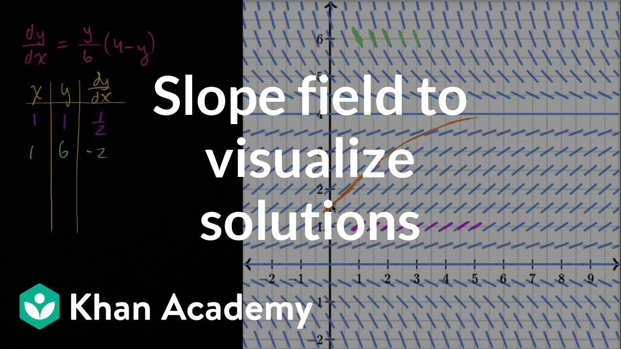
Slope field to visualize solutions | First order differential equations | Khan Academy
Calculus 1: Slope Fields Examples

The Theory of 2nd Order ODEs // Existence & Uniqueness, Superposition, & Linear Independence
Euler's Method (introduction & example)

Matching Slope Fields to Differential Equations Part 2
5.0 / 5 (0 votes)
Thanks for rating: