Calculus AB Homework 7.2 Slope Fields
TLDRThis video tutorial guides viewers through solving unit 7 homework problems 13 to 20, focusing on slope fields for differential equations. It demonstrates how to sketch slope fields by identifying key points where the derivative equals zero or specific values like 1, and uses patterns to fill in the fields. The video also explains how to find particular solutions to given differential equations using initial conditions, showcasing the process of separating variables and integrating to solve for y.
Takeaways
- 📚 The video is a tutorial on solving differential equations by sketching slope fields for various equations.
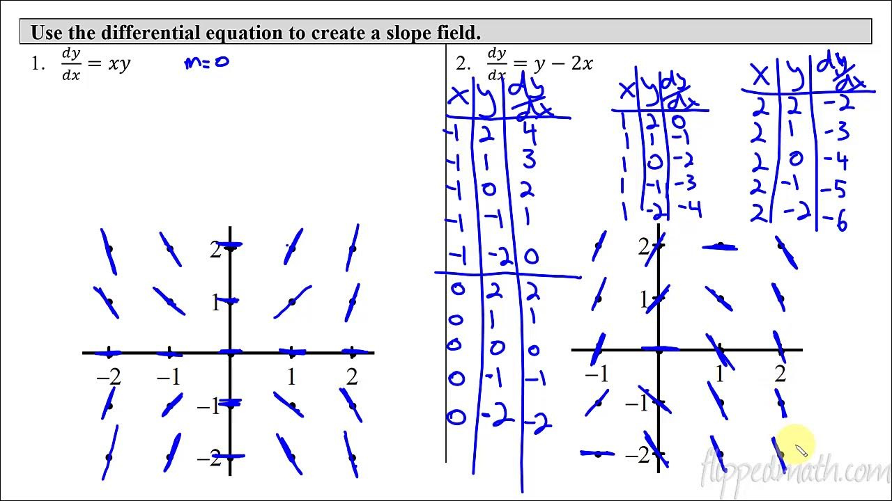
- 🔍 The process begins by identifying points where the slope is zero, such as when x and y have opposite values or are both zero.
- 📈 The tutorial demonstrates how to determine the slope at specific points, like (1,0) and (2,-1), by setting the differential equation equal to zero.
- 📝 The importance of visualizing slopes, such as a 45-degree angle for a slope of 1, is emphasized for easier sketching.
- 🔑 The video uses symmetry and patterns to simplify the process of drawing the slope field, like drawing parallel lines for the same slope values.
- 🤔 The presenter considers the behavior of the slope field at the axes and points of discontinuity, such as vertical tangents at x = 0 when y ≠ 0.
- 📉 For equations like dy/dx = x - y, the slope field is determined by the relationship between x and y, with slopes being 1 when x is one more than y.
- 📌 The video explains how to find particular solutions to differential equations using initial conditions, by separating variables and integrating.
- 📐 The tutorial covers various types of differential equations, including those with no y term, which simplifies the slope field to being dependent only on x.
- 📈 The process of sketching slope fields involves estimating the steepness of slopes and drawing lines accordingly, which can be subjective and challenging.
- 🔚 The video concludes with finding particular solutions for given initial conditions by substituting values into the general solution and solving for the constant.
Q & A
What is the main topic of the video?
-The main topic of the video is working through unit 7 homework problems 13 through 20, which deal with slope fields and differential equations.
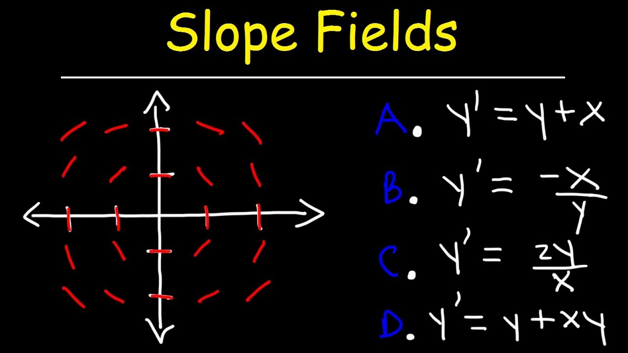
How does the video approach the problem of drawing a slope field for the differential equation dy/dx = x + y?
-The video suggests starting by identifying points where the derivative equals zero and then moving on to points where the slope is 1, using these to establish patterns and visualize the slope field.
What is the significance of the point (0,0) in the context of the differential equation dy/dx = x + y?
-At the point (0,0), the slope is 0 because the x and y values are equal and opposite, satisfying the condition for the slope to be zero in the given differential equation.
How does the video illustrate the process of drawing a slope field for dy/dx = x - y?
-The video explains that the slope field for dy/dx = x - y can be drawn by identifying points where the slope is 0, such as (0,0) and (1,1), and then determining the slope for other points based on the x and y values.
What is the pattern observed for the slope field of dy/dx = -y/x?
-The pattern observed is that when x and y have the same value, the slope is -1, and when they are opposite, the slope is +1. Additionally, when y is 0, the slope is 0, except at the origin (0,0) where it is undefined.
How does the video handle the differential equation dy/dx = x * y?
-The video suggests that at points where x is 0, the slope is 0 regardless of the y value. It also shows that the slope increases linearly with the y value when x is a constant non-zero value.
What is the initial slope for the differential equation dy/dx = x + 1?
-The initial slope for the differential equation dy/dx = x + 1 is 1, as there is no y term in the slope equation, making the slope purely determined by the x coordinate.
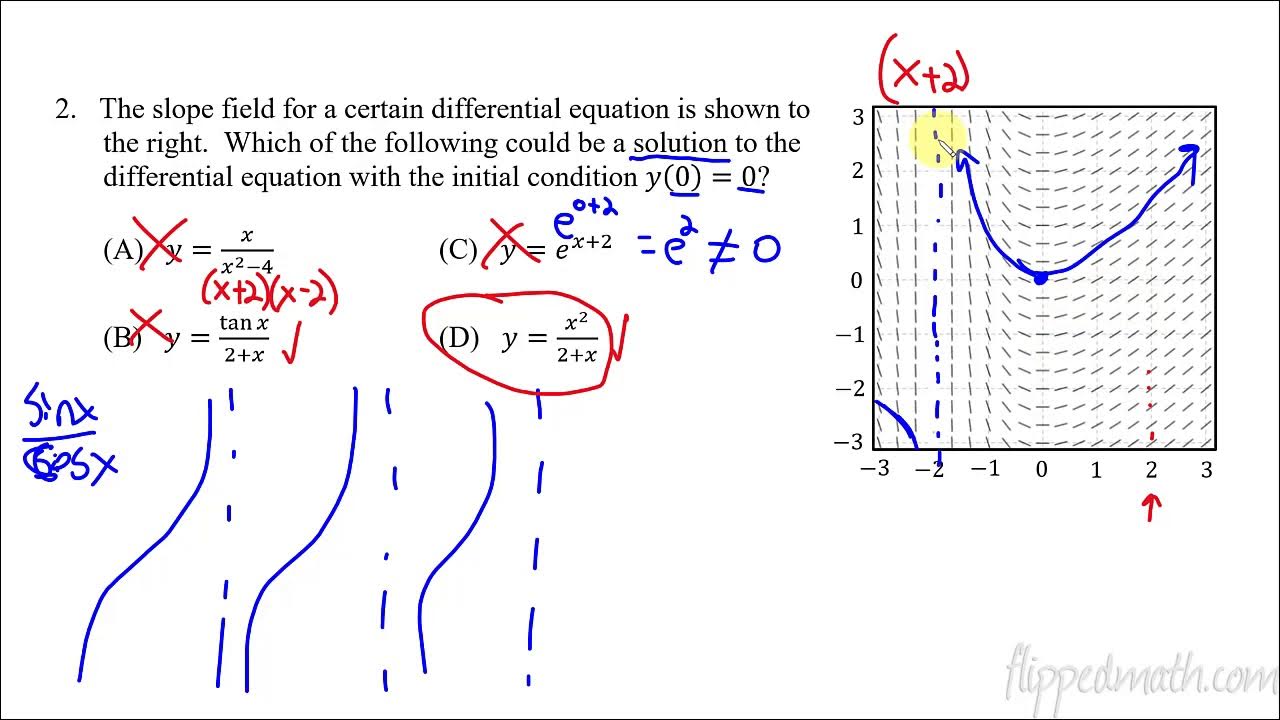
How does the video explain the slope field for dy/dx = 1/(x+1)?
-The video explains that the slope field for dy/dx = 1/(x+1) will have a slope of 1 at x=0, slopes decreasing as x increases, and vertical tangents (undefined slopes) at x=-1.
What is the method used in the video to find a particular solution to the differential equation dy/dx = x^2 * y - 1 with the initial condition y(0) = 3?
-The video uses separation of variables, followed by integration and exponentiation to find the general solution, and then applies the initial condition to find the particular solution.
How does the video describe the points in the XY plane for which the slopes are positive for the differential equation dy/dx = x^2 * y - 1?
-The video describes that the slopes are positive for points in the XY plane where x is not 0 and y is greater than 1, as this is when y - 1 is positive, resulting in a positive slope.
What is the general solution found in the video for the differential equation dy/dx = x^4 * y - 2?
-The general solution found in the video for the differential equation dy/dx = x^4 * y - 2 is y = 2 - 2 * e^(x^5/5), after applying separation of variables and integration.
Outlines
📚 Introduction to Unit 7 Homework - Slope Fields
The script begins with an introduction to the homework problems for Unit 7, focusing on slope fields for differential equations. The first problem involves drawing a slope field for the equation dy/dx = x + y, starting with points where the slope equals zero, then moving to points with a slope of one, and observing patterns along diagonals. The process involves visualizing the slope at various points and drawing lines with the corresponding steepness.
🔍 Analyzing Slope Patterns in Differential Equations
This paragraph continues the exploration of slope fields, examining different scenarios for the differential equation dy/dx = x - y. The speaker discusses the slope at specific points, such as (0,0), (1,1), and (2,2), and identifies patterns where the slope equals one when the x-coordinate is one more than the y-coordinate. The process includes correcting previous drawings to ensure accuracy and consistency in the representation of slopes.
📉 Sketching Slope Fields with Varying Differential Equations
The script proceeds with the analysis of different differential equations, such as dy/dx = -y/x, and the corresponding slope fields. The discussion includes the behavior of slopes when x and y have the same or opposite values, and the identification of vertical slopes when the y-coordinate is zero. The speaker also explores the symmetry in the slope field and the reflection of patterns across axes.
📈 Complex Slope Fields and Initial Conditions
The fourth paragraph delves into more complex slope fields, such as dy/dx = x * y and dy/dx = x + 1, and the challenges of distinguishing between steep slopes. The speaker also addresses the process of finding particular solutions to differential equations using initial conditions, such as y(0) = 3, and the method of separation of variables to solve the equations.
🧩 Solving Differential Equations with Initial Conditions
This section focuses on solving a specific differential equation, dy/dx = x^4 * y - 2, with an initial condition of y(0) = 0. The process involves separating variables, integrating both sides, and applying the initial condition to find the particular solution. The speaker also describes how to identify points in the xy-plane where the slopes are negative.
📘 Final Thoughts on Slope Fields and Differential Equations
The final paragraph wraps up the discussion on slope fields, summarizing the process of sketching slope fields for the given differential equations and finding particular solutions with initial conditions. The speaker emphasizes the importance of understanding the behavior of slopes and the application of mathematical techniques to solve differential equations.
Mindmap
Keywords
💡Slope field
💡Differential equation
💡Derivative
💡Ordered pair
💡Diagonal
💡Steepness
💡Separation of variables
💡Initial condition
💡Integration
💡Exponentiation
💡Absolute value
Highlights
Introduction to drawing slope fields for differential equations in Unit 7 homework problems 13 through 20.
Method to determine when the derivative equals zero by analyzing the differential equation for patterns.
Visualizing a 45-degree angle as a slope of 1 for easier drawing on the slope field.
Observation of diagonal patterns in slope fields where slopes are the same.
Drawing slope fields for the differential equation dy/dx = x - y, noting the slope at specific points.
Identification of vertical slopes and undefined slopes in the slope field for dy/dx = -y/x.
Symmetry in slope fields allowing for reflection across axes to simplify drawing.
Challenges in distinguishing steep slopes in the slope field for dy/dx = x * y.
Slope determination for dy/dx = x + 1, highlighting the independence of y on the slope.
Analysis of slope fields for dy/dx = 1/(x+1), including vertical tangents at specific points.
Sketching a slope field for dy/dx = x^2 * y - 1 at 12 indicated points.
Describing regions in the XY plane with positive slopes for the differential equation in Part B.
Finding a particular solution to the differential equation with an initial condition in Part C.
Drawing a slope field for dy/dx = x^4 * y - 2 and identifying points with negative slopes.
Solving for a particular solution to the differential equation with an initial condition of f(0) = 0.
General strategies for solving differential equations and finding particular solutions.
The importance of understanding the relationship between the differential equation and the slope field.
Practical applications of slope fields in visualizing the behavior of solutions to differential equations.
Transcripts


5.0 / 5 (0 votes)
Thanks for rating: