Area Between Two Curves!
TLDRIn this informative video, the presenter delves into the mathematical concept of finding the area between two curves, a topic that is integral to calculus. The method involves setting up an integral that represents the difference between the top and bottom functions over a given interval, which is bounded by vertical lines corresponding to specific x-values. The presenter illustrates this with examples, such as finding the area between x^2 and x from x=0 to x=1, and between 1/x and x^3 from x=1 to x=3. Additionally, the video addresses the challenge of determining when the roles of the top and bottom functions switch, which may require multiple integrals. The presenter also introduces the application of this concept to business, specifically in calculating consumer and producer surplus in a market. The video concludes with a reminder of the importance of maintaining the top-minus-bottom relationship in the integral and encourages viewers to practice these techniques for a deeper understanding.
Takeaways
- 📐 **Integration for Area Between Curves**: To find the area between two curves, integration is used, specifically the integral from the lower to the upper function over a given interval.
- 🔍 **Defining the Area**: The area of interest is determined by the bounds defined by two vertical lines, x=a and x=b, which correspond to the points where the area is to be calculated.
- 🛠️ **Subtracting for Total Area**: The total area between the curves is found by subtracting the area under the lower curve (G(x)) from the area under the upper curve (f(x)).
- 📈 **Combining Integrals**: When the bounds of integration are the same for both curves, the integrals can be combined into a single integral of the top function minus the bottom function over the interval [a, b].
- 📉 **Visualizing with Graphs**: Graphing calculators or software can be helpful to visualize the area between curves and to determine which function is on top or bottom within a given interval.
- 🔢 **Solving for Endpoints**: When endpoints are not given, they can be found by setting the two functions equal to each other and solving for x.
- 🔄 **Switching Functions**: If the roles of the top and bottom functions switch within the interval, it may be necessary to compute multiple integrals to account for the different sections.
- 🧮 **Evaluating Definite Integrals**: The definite integral is evaluated by applying the antiderivative of the expression (top function minus bottom function) and then using the Fundamental Theorem of Calculus.
- 💰 **Business Application**: The concepts can be applied to business scenarios, such as calculating consumer and producer surplus through the areas between demand and supply curves.
- ⚖️ **Consumer and Producer Surplus**: Consumer surplus is the area above the demand curve and below the equilibrium price, while producer surplus is the area below the supply curve and above the equilibrium price.
- 🔧 **Equilibrium Point**: To find consumer and producer surplus, one must first determine the equilibrium point where the supply and demand curves intersect.
Q & A
What is the general method to find the area between two curves?
-The general method to find the area between two curves involves integration. Specifically, you calculate the integral from the left bound to the right bound of the top function minus the bottom function with respect to x.
How does one determine the bounds for the integral when finding the area between two curves?
-The bounds for the integral are typically given as lines x equals a and x equals b, which represent the horizontal boundaries of the area you're interested in. If not given, you may need to find the points of intersection where the two curves meet to determine these bounds.
What is the formula for calculating the area between two curves?
-The formula for calculating the area between two curves is the integral from A to B of (f(x) - g(x)), where f(x) is the top function and g(x) is the bottom function, and A and B are the bounds of integration.
How do you find the area between the curves y = x^2 and y = x between x = 0 and x = 1?
-To find the area between y = x^2 and y = x between x = 0 and x = 1, you would calculate the integral from 0 to 1 of (x - x^2) with respect to x. Upon solving, the result is (1/2 - 1/3), which simplifies to 1/6.
What is the significance of maintaining the 'top minus bottom' relation when calculating the area between two curves?
-Maintaining the 'top minus bottom' relation is crucial because it ensures that you are correctly calculating the area between the two curves and not including any part of the area that lies below the bottom curve or above the top curve.
How can you find the endpoints of integration without a graphing calculator?
-Without a graphing calculator, you can find the endpoints of integration by setting the two functions equal to each other and solving for x. Additionally, you can use test points within the suspected interval to determine which function is on top and which is on the bottom.
What is consumer surplus and how is it represented graphically?
-Consumer surplus is the difference between the maximum price a consumer is willing to pay for a good and the actual price they pay. Graphically, it is represented by the area between the demand curve and the price consumers pay up to the equilibrium quantity.
What is producer surplus and how is it calculated?
-Producer surplus is the difference between the minimum price a producer is willing to accept for a good and the actual price they receive. It is calculated by integrating from the equilibrium quantity to zero of the equilibrium price minus the supply function with respect to x.
How do you find the equilibrium point in a market characterized by a supply and demand curve?
-The equilibrium point is found by setting the supply and demand functions equal to each other and solving for the equilibrium quantity (x). Once the equilibrium quantity is found, the equilibrium price (P) can be determined by substituting the equilibrium quantity into either the supply or demand function.
What is the business application of finding the area between two curves?
-The business application of finding the area between two curves is often related to calculating consumer and producer surplus in a market. These areas represent the economic benefits to consumers and producers, respectively, at the equilibrium point of a market.
Why is it important to have a graphing calculator when dealing with finding areas between curves?
-A graphing calculator is important because it allows you to visualize the curves, their intersections, and the areas in question. This can make it much easier to determine the correct setup for the integral, especially when dealing with curves that switch positions (top to bottom and vice versa) across different intervals.
Outlines
📐 Introduction to Finding Area Between Two Curves
The video begins with an introduction to calculating the area between two curves, which is expected to involve integration, as it is similar to finding the area under a single curve. The presenter draws two functions, f(x) and g(x), and illustrates how to find the area between them bounded by the lines x=a and x=b. The method involves subtracting the integral of the lower function g(x) from the integral of the upper function f(x) between the bounds a and b. The general formula for this calculation is presented, and the importance of maintaining the order of integration (top function minus bottom function) is emphasized.
📈 Example Calculation: Area Between f(x) = x^2 and g(x) = x
The presenter provides a step-by-step example of finding the area between the curves f(x) = x^2 and g(x) = x, bounded by x=0 and x=1. A graphing calculator is suggested for visual aid. The integral of the upper function minus the integral of the lower function is calculated, resulting in the area being (1/2)x^2 - (1/3)x^3, evaluated from 0 to 1. The final answer is obtained by substituting the bounds into the antiderivative, resulting in 1/6 as the area between the curves.
🔍 Finding Endpoints and Determining Top/Bottom Functions
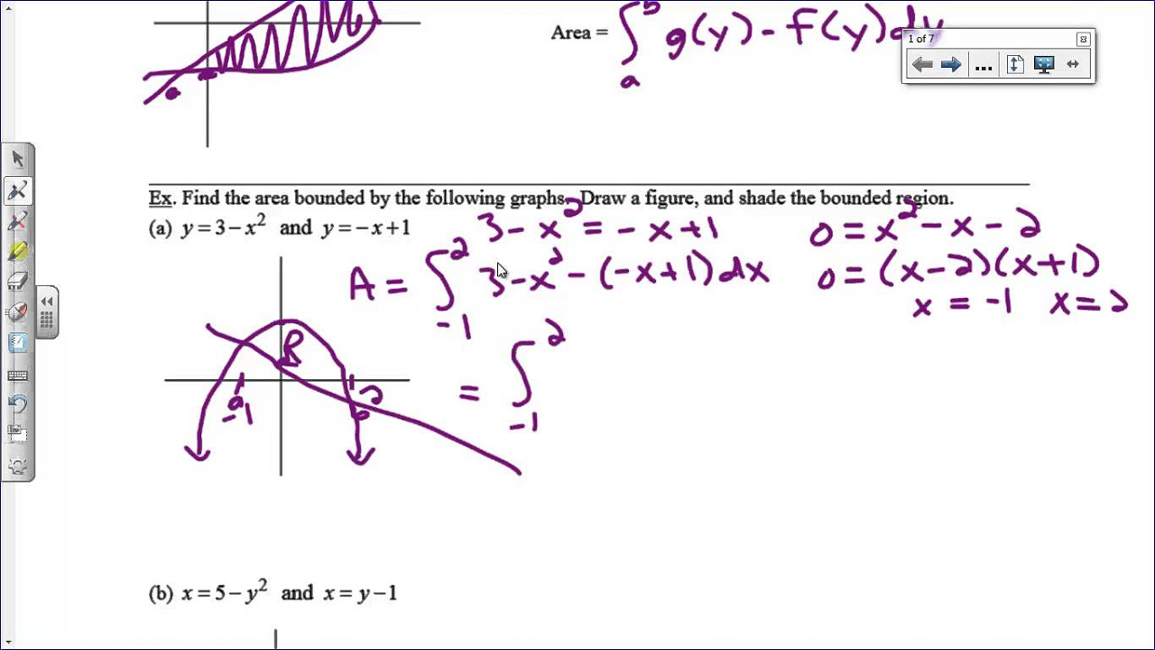
The video discusses how to find the endpoints for integration when they are not given, by setting the two functions equal to each other. It also covers how to determine which function is the top and which is the bottom without a graphing calculator, using test points. An example is given with the functions y = 5x - x^2 and y = x, where the endpoints are found by solving the equation 5x - x^2 = x. The presenter also demonstrates how to calculate the area between these functions using integration, resulting in an area of 32/3.
🛠️ Dealing with Functions that Switch Places: Multiple Integrals
The video addresses the scenario where the top and bottom functions switch places, which requires setting up multiple integrals to account for different sections where each function is on top. An example is given with the functions f(x) = x^3 - x and g(x) = 0, which intersect at points that necessitate two separate integrals, I1 and I2. The presenter shows how to find the endpoints by solving the equation x^3 - x = 0 and how to use test points to determine the top and bottom functions in different regions. The final area is the sum of the two integrals, calculated separately for each region.
💼 Business Application: Consumer and Producer Surplus
The presenter introduces a business application of finding the area between two curves, specifically in the context of consumer and producer surplus. The concept of surplus is explained using an example of a transaction involving a phone, where the difference between the selling price and the seller's willingness to accept and the buyer's willingness to pay represents the producer and consumer surplus, respectively. The video then demonstrates how to calculate these surpluses using integration, with the consumer surplus being the integral from the equilibrium quantity to zero of the demand function minus the price, and the producer surplus being the integral from zero to the equilibrium quantity of the price minus the supply function.
🧮 Example Calculations of Consumer and Producer Surplus
The video concludes with an example calculation of consumer and producer surplus using given demand and supply functions. The equilibrium point is found by equating the supply and demand functions, and then the equilibrium price is determined by substituting the equilibrium quantity into either function. The producer surplus is calculated by integrating from zero to the equilibrium quantity of the equilibrium price minus the supply function, resulting in $13.72. Similarly, the consumer surplus is calculated by integrating from zero to the equilibrium quantity of the demand function minus the equilibrium price, resulting in $35.28. The video emphasizes the importance of maintaining the order of functions when integrating and the practical application of these calculations in economics.
Mindmap
Keywords
💡Integration
💡Area Between Curves
💡Bounds of Integration
💡Top Function and Bottom Function
💡Definite Integral
💡Consumer Surplus and Producer Surplus
💡Equilibrium Point
💡Supply and Demand Functions
💡Power Rule
💡Graphing Calculator
💡Endpoints
Highlights
The area between two curves can be found using integration, specifically the integral from the left to right bounds of the top function minus the bottom function.
To find the total area between two curves, subtract the area under the bottom curve from the area under the top curve.
When the top and bottom functions switch places, you may need more than one integral to find the total area between them.
Use a graphing calculator to easily determine the top and bottom functions and their intersection points.
If no graph is provided, test points can be used to determine which function is on top between intersection points.
Always maintain the top minus bottom relation when setting up the integral to find the area between curves.
The area between curves has a business application in finding consumer and producer surplus.
Consumer surplus is the difference between what consumers are willing to pay and the equilibrium price.
Producer surplus is the difference between the equilibrium price and what producers are willing to accept.
Find consumer surplus by integrating the demand function minus the price from 0 to the equilibrium quantity.
Find producer surplus by integrating the price minus the supply function from 0 to the equilibrium quantity.
To find the equilibrium quantity and price, set the demand and supply functions equal to each other and solve for x and the price respectively.
Always show your work, especially when finding endpoints and determining which function is on top.
These area between curves problems can be tedious but are a lot of fun with practice.
Remember to always plug in the equilibrium quantity into either the demand or supply function to find the equilibrium price.
The answers for consumer and producer surplus are in dollars, representing the extra money or surplus.
Set up the integral correctly with top minus bottom and maintain this relation throughout the problem.
Finding the area between curves is a fundamental concept with applications in business and economics.
Transcripts
Browse More Related Video
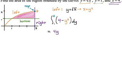
Area Between Curves: Integrating with Respect to y (Example 3)

Area Between Two Curves

Area Between Curves: Integrating with Respect to y (Example 2)
Area of a Region Between Two Curves
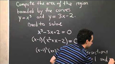
Area Between y=x^3 and y=3x-2 | MIT 18.01SC Single Variable Calculus, Fall 2010
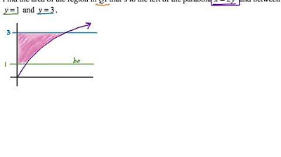
Area Between Curves: Integrating with Respect to y (Example 1)
5.0 / 5 (0 votes)
Thanks for rating: