Midpoint Rule & Riemann Sums
TLDRThis video tutorial explains the midpoint rule for approximating the area under a curve. It uses two examples: y=x^2 from 0 to 8 and y=x^3 from 0 to 10. The process involves dividing the interval into subintervals, calculating the midpoint of each, and summing the product of the delta x and the y-values at these points. The results are then compared to the exact areas found using definite integrals, demonstrating the midpoint rule's effectiveness in estimation.
Takeaways
- 📈 The video discusses the application of the midpoint rule for estimating areas under a curve, specifically using the function y = x^2 from 0 to 8 and y = x^3 from 0 to 10.
- 📊 The midpoint rule involves dividing the interval under consideration into subintervals and calculating the area of rectangles based on the midpoints of these subintervals.
- 🔢 The formula for the length of each sub-interval (delta x) is given by (b - a) / n, where a and b are the endpoints of the interval and n is the number of subintervals.
- 🏢 The area under the curve is approximated by summing the heights of the rectangles (width times height) and multiplying by delta x.
- 🏗️ In the first example with y = x^2, the area is estimated by finding the midpoints at 1, 3, 5, and 7 and calculating the area as 168 using the midpoint rule.
- 🔍 The exact area under the curve for y = x^2 from 0 to 8 is found by evaluating the definite integral, which results in an actual area of 170.67.
- 🏢 For the second example with y = x^3, the area is estimated by finding the midpoints at 1, 3, 5, 7, and 9 and calculating the area as 2450 using the midpoint rule.
- 🔍 The exact area under the curve for y = x^3 from 0 to 10 is calculated by evaluating the definite integral, resulting in an actual area of 2500.
- 💡 The midpoint rule provides a good approximation of the actual area under a curve, especially when compared to using left or right endpoints.
- 📚 It is recommended to watch additional videos on Riemann sums, left endpoints, and right endpoints for a deeper understanding of the concepts.
- 👍 The video script serves as a practical guide for using the midpoint rule to estimate areas under curves and highlights its effectiveness in approximating definite integrals.
Q & A
What is the main topic of the video?
-The main topic of the video is explaining the midpoint rule and its application in approximating the area under a curve.
How is the graph of y equals x squared described in the video?
-The graph of y equals x squared is described as a curve that the video focuses on the right side of, to determine the area under it from 0 to 8.
What is the formula used to calculate the length of each sub-interval in the midpoint rule?
-The formula used to calculate the length of each sub-interval, denoted as delta x, is (b - a) / n, where a and b are the endpoints of the interval, and n is the number of sub-intervals.
How many sub-intervals are used to approximate the area under the curve of y equals x squared from 0 to 8 in the video?
-Four sub-intervals are used to approximate the area under the curve in the given example.
What is the midpoint rule's approach to estimate the area under a curve?
-The midpoint rule estimates the area under a curve by drawing rectangles on the curve with their heights at the midpoint of each sub-interval and then calculating the area of these rectangles to approximate the total area under the curve.
How is the area calculated for each rectangle in the midpoint rule?
-The area for each rectangle is calculated by multiplying the width (delta x) by the height (the y value at the midpoint of the sub-interval).
What is the exact area under the curve of y equals x squared from 0 to 8, and how does it compare to the midpoint rule approximation?
-The exact area under the curve is calculated as the definite integral from 0 to 8 of x squared, which is (8^3)/3 - (0^3)/3, resulting in 170.67. The midpoint rule approximation yields 168, showing a close match to the exact value.
What is the second function discussed in the video for approximating the area under the curve?
-The second function discussed is y equals x to the third power, for estimating the area under the curve over the closed interval from 0 to 10.
How many sub-intervals are chosen for the approximation of the area under the curve of y equals x cubed from 0 to 10?
-Five sub-intervals are chosen for the approximation in the given example.
What is the exact area under the curve of y equals x cubed from 0 to 10, and how does it compare to the midpoint rule approximation?
-The exact area is calculated as the definite integral from 0 to 10 of x cubed, which is (10^4)/4 - (0^4)/4, resulting in 2500. The midpoint rule approximation yields 2450, again showing a close match to the exact value.
What can the midpoint rule be used for?
-The midpoint rule can be used to estimate the value of a definite integral, providing a good approximation of the area under a curve.
Outlines
📊 Introduction to the Midpoint Rule
This paragraph introduces the concept of the midpoint rule and its application in calculating the area under a curve. It begins with a discussion on the graph of y equals x squared and focuses on the right side of the graph. The midpoint rule is used to estimate the area under the curve from 0 to 8 by dividing the interval into four subintervals. The formula for calculating the length of each sub-interval (delta x) is provided. The video emphasizes the importance of understanding left and right endpoints and Riemann sums, suggesting viewers watch previous videos for a better grasp of these concepts. The midpoint rule is shown to be a good approximation for estimating the area under the curve compared to using left or right endpoints.
📈 Application of the Midpoint Rule with y = x^2
The paragraph delves into the practical application of the midpoint rule using the function y equals x squared. It explains the process of drawing rectangles based on the midpoints of subintervals and calculating the area of these rectangles to approximate the area under the curve. The specific midpoints used (1, 3, 5, and 7) are calculated, and the corresponding y-values (squared numbers) are summed up to estimate the area. The paragraph then compares this approximation to the exact area calculated using the definite integral, demonstrating the accuracy of the midpoint rule. The process is detailed step-by-step, providing a clear understanding of how the midpoint rule can be applied to estimate areas under curves.
🔢 Midpoint Rule Applied to x^3 Function
In this paragraph, the midpoint rule is applied to a different function, x to the power of three, over the closed interval from 0 to 10. The process involves dividing the interval into five subintervals and calculating the midpoint of each to estimate the area under the curve. The y-values corresponding to these midpoints are found by cubing the x-values, and the sum of these values is multiplied by the delta x to estimate the area. The paragraph then compares this approximation with the actual area calculated using the definite integral of x cubed from 0 to 10. The comparison shows that the midpoint rule provides a close approximation of the actual area, reinforcing its utility in estimating integrals.
Mindmap
Keywords
💡Midpoint Rule
💡Graph
💡Area Under the Curve
💡Subintervals
💡Delta X
💡Antiderivatives
💡Definite Integral
💡Approximation
💡Function Values
💡Power Rule
💡Integration
Highlights
Introduction to the concept of using the midpoint rule for estimating the area under a curve.
Graphing the function y = x^2 and focusing on its right side for demonstration.
Explanation of breaking the area under the curve into four subintervals for calculation.
Using the formula delta x = (b - a) / n to calculate the length of each sub-interval.
Calculation of delta x for the interval from 0 to 8, resulting in a value of 2.
Recommendation to watch a previous video on Riemann sums for better understanding.
Process of drawing four rectangles using the midpoint rule on the graph.
Explaining the approximation of the area under the curve by the midpoint rule.
The method of calculating the area of each rectangle using its width and height.
Detailing the summing of individual rectangle heights to calculate total area.
Comparison of midpoint rule with left and right endpoint methods for approximation.
Using specific examples to demonstrate the calculation of areas using the midpoint rule.
Contrasting the approximation by the midpoint rule with the exact area calculation using definite integrals.
Introducing a new example with the function x^3 to apply the midpoint rule.
Calculating the area under the curve for x^3 using the midpoint rule and comparing it to the definite integral.
Concluding remarks on the effectiveness of the midpoint rule for estimating the area under curves.
Transcripts
Browse More Related Video
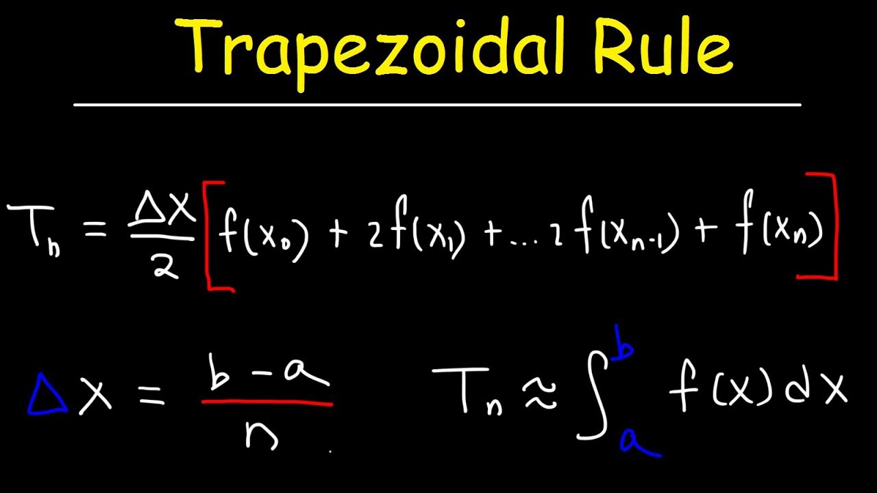
Trapezoidal Rule
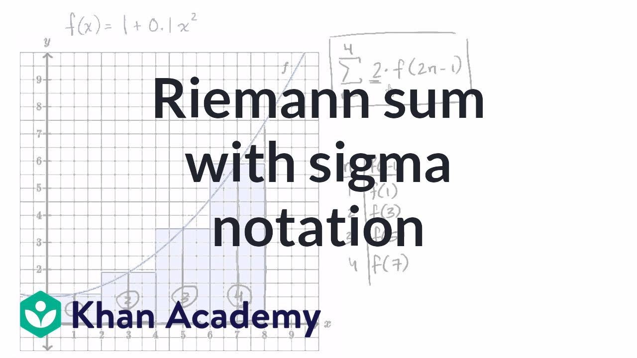
Worked example: Riemann sums in summation notation | AP Calculus AB | Khan Academy
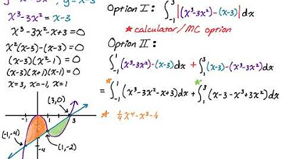
Area Between Two Curves with Multiple Regions: y = x^3-3x^2 and y = x-3
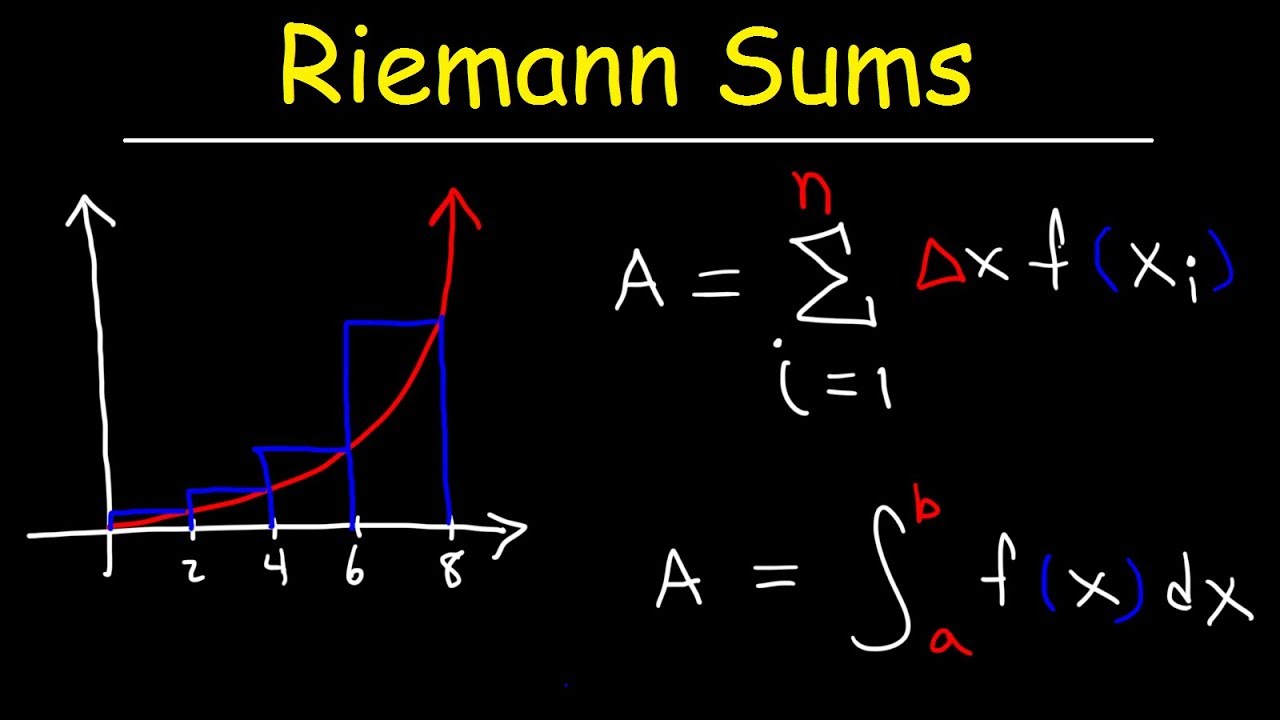
Riemann Sums - Left Endpoints and Right Endpoints

Riemann approximation introduction | Accumulation and Riemann sums | AP Calculus AB | Khan Academy
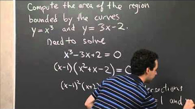
Area Between y=x^3 and y=3x-2 | MIT 18.01SC Single Variable Calculus, Fall 2010
5.0 / 5 (0 votes)
Thanks for rating: