Applications of Slope Fields (Differential Equations 10)
TLDRThe transcript delves into the application of slope fields in real-life scenarios, particularly focusing on the dynamics of air resistance and gravity on falling objects, leading to the concept of terminal velocity. It further explores the population growth model, highlighting the impact of resources on population size and the emergence of carrying capacity. The discussion emphasizes the practical insights slope fields offer in understanding complex systems without the need for precise mathematical solutions.
Takeaways
- 📈 Slope fields are graphical representations that show how the rate of change of a system varies at different points.
- 🚀 The concept is applied to model real-life situations, such as the effect of wind resistance on a falling object.
- 💨 Wind resistance acts as an upward force that opposes gravity, affecting the acceleration and terminal velocity of a falling object.
- 📉 In the presence of air resistance, the acceleration of a falling object decreases as its velocity increases due to the increasing opposing force.
- 🏆 Terminal velocity is the constant speed that a falling object reaches when the force of air resistance equals the force of gravity.
- 🔢 The mathematical model for terminal velocity is derived by setting the gravitational acceleration minus the air resistance (proportional to velocity) equal to zero.
- 📊 Slope fields can be used to visualize and understand the dynamics of population growth and carrying capacity.
- 🌿 Carrying capacity is the maximum population size that can be sustained in a given environment without resource depletion.
- 📈 A population's growth rate starts high when the population is low but slows down as it approaches the carrying capacity.
- 📉 If the initial population exceeds the carrying capacity, the population will decline due to limited resources.
- 🔄 Slope fields provide insights into the behavior of dynamic systems without the need for explicit solutions to the differential equations.
- 🛠️ Slope fields are a tool for understanding trends and equilibrium points in systems, which can be applied to various fields such as physics and ecology.
Q & A
What is the main concept discussed in the transcript?
-The main concept discussed in the transcript is the application of slope fields in understanding and modeling real-life problems using differential equations, specifically focusing on scenarios involving gravitational acceleration and air resistance, as well as population dynamics and carrying capacity.
How does air resistance affect the acceleration of a falling object?
-Air resistance affects the acceleration of a falling object by counteracting the force of gravity. As the object's velocity increases due to gravity, it encounters more air resistance, which acts as an upward force. Eventually, the air resistance becomes equal to the gravitational force, resulting in a net acceleration of zero, which is when the object reaches its terminal velocity and no longer accelerates.
What is the formula used to represent air resistance in the context of the transcript?
-In the context of the transcript, air resistance is represented by the formula K*V, where K is a proportionality constant based on the object's properties and V is the velocity of the object.
How does the concept of terminal velocity relate to the discussion in the transcript?
-Terminal velocity is the constant speed that a freely falling object eventually reaches when the resistance of the air is equal to the force of gravity acting on the object. In the transcript, it is discussed as the point at which the acceleration of the falling object becomes zero due to air resistance balancing out the gravitational pull.
What is the role of slope fields in modeling real-life problems?
-Slope fields play a crucial role in modeling real-life problems by providing a visual representation of how a system's state changes over time. They allow us to understand the dynamics of the system without necessarily solving the differential equations analytically. By examining the slopes at different points, we can infer trends, such as increasing or decreasing rates, and equilibrium points in the system.
How does the transcript relate the concept of slope fields to population dynamics?
-The transcript relates slope fields to population dynamics by discussing how the growth or decline of a population can be modeled using differential equations. The rate of population change is represented by the slope at different population levels, which can reveal insights about the carrying capacity and how a population will behave over time when resources are limited.
What is the term used in the transcript to describe the maximum population size that can be sustained indefinitely?
-The term used in the transcript to describe the maximum population size that can be sustained indefinitely is 'carrying capacity'.
How does the transcript illustrate the balance between gravity and air resistance?
-The transcript illustrates the balance between gravity and air resistance through the concept of terminal velocity. It explains that as a falling object gains speed due to gravity, it also encounters increasing air resistance. When the air resistance equals the gravitational force, the object stops accelerating and continues to fall at a constant speed, known as terminal velocity.
What is the significance of the equilibrium solution in the context of the transcript?
-In the context of the transcript, the equilibrium solution is significant because it represents the stable state of a system where there is no net change. For example, in the case of population dynamics, the equilibrium solution (carrying capacity) is the population size where the growth rate is zero, meaning the population will neither increase nor decrease if it remains at that level.
How does the transcript demonstrate the use of slope fields in understanding system behavior?
-The transcript demonstrates the use of slope fields by providing examples of how they can visualize the behavior of systems described by differential equations. By examining the slopes at various points, one can predict how the system will evolve over time, whether it will reach an equilibrium, grow indefinitely, or eventually decline.
Outlines
📚 Introduction to Slope Fields and Real-Life Applications
This paragraph introduces the concept of slope fields and their application to real-life problems, particularly focusing on the use of differential equations. It discusses the transition from simplistic models that neglect factors like wind resistance to more complex ones that incorporate these elements. The example of a person jumping out of a helicopter is used to illustrate how air resistance affects the acceleration and velocity of a falling object, highlighting the interplay between gravity and air resistance.
🚀 Terminal Velocity and the Role of Air Resistance
The paragraph delves into the concept of terminal velocity, explaining how it is reached when the force of air resistance equals the force of gravity. It describes the process of an object falling and gaining velocity until air resistance becomes significant enough to counteract gravity, resulting in a constant velocity. The mathematical relationship between gravitational acceleration, air resistance, and velocity is explored, with a specific example given involving a constant of proportionality for air resistance.
📈 Visualizing Slope Fields for Velocity and Air Resistance
This section discusses the visualization of slope fields to represent the situation of an object falling with air resistance. It explains how to create a slope field based on the first-order differential equation that describes the relationship between gravitational acceleration and air resistance. The paragraph provides a step-by-step guide on plugging in values for velocity at different times to determine the slope of the field, which in turn illustrates how the velocity of the object changes over time.
🌬️ Air Resistance and Velocity: A Dynamic Balance
The paragraph continues the discussion on air resistance and its impact on the velocity of a falling object. It explains how the rate of change of velocity (acceleration) is affected by the increasing air resistance as the object's speed increases. The concept of terminal velocity is reinforced, emphasizing that once this velocity is reached, the object will not change speed anymore regardless of its initial velocity. The paragraph also introduces the idea of a slope field video that was mentioned previously, hinting at a visual aid for understanding these concepts.
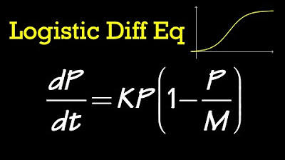
📊 Slope Fields and Population Dynamics
This paragraph shifts the focus to population dynamics and how slope fields can be used to model changes in population over time. It introduces the concept of carrying capacity, which is the maximum population size that can be sustained in a given environment. The paragraph explains how the rate of population growth (or decline) is influenced by the current population size and the available resources, using the example of a pond with fish to illustrate the point.
🌿 Carrying Capacity and Population Growth
The paragraph further explores the idea of carrying capacity and its implications for population growth. It describes how populations start growing slowly when they are low due to limited resources, but as the population increases, the growth rate accelerates until it reaches a point where the resources are fully utilized, and the growth rate slows down again. The concept of an equilibrium solution is introduced, where the population stabilizes at the carrying capacity, regardless of the starting point.
🔍 Interpreting Slope Fields and Real-Life Trends
The final paragraph summarizes the key takeaways from the discussion on slope fields and their applications to real-life scenarios. It emphasizes the ability to understand trends in population growth or velocity changes without having to solve the underlying differential equations. The paragraph highlights the usefulness of slope fields in providing insights into limiting factors and equilibrium solutions, and it sets the stage for future discussions on determining the existence and uniqueness of solutions in differential equations.
Mindmap
Keywords
💡Slope Fields
💡Differential Equations
💡Terminal Velocity
💡Air Resistance
💡Gravity
💡Velocity
💡Acceleration
💡Carrying Capacity
💡Equilibrium Solution
💡First Derivative
Highlights
Introduction to slope fields and their application in solving real-life problems using differential equations.
Discussion on the unrealistic nature of neglecting factors like wind resistance in simplified word problems.
Explanation of how wind resistance affects the acceleration of a falling object.
Derivation of the relationship between gravitational acceleration, air resistance, and terminal velocity.
Illustration of the concept of terminal velocity with a practical example of jumping out of a helicopter.
Construction of a slope field to describe the situation of falling objects with air resistance.
Demonstration of how the slope field changes with different initial velocities.
Explanation of the equilibrium solution in the context of terminal velocity.
Application of slope fields to population dynamics and the concept of carrying capacity.
Discussion on how population growth is influenced by available resources and carrying capacity.
Use of slope fields to predict population trends and equilibrium points without solving the differential equation.
Interpretation of real-life situations using slope fields, such as population growth and resource limitations.
Explanation of how slope fields can provide insights into the behavior of systems without the need for exact solutions.
The importance of understanding the implications of slope fields in modeling real-world phenomena.
Overview of the next topic, which involves determining when unique solutions exist for differential equations.
Transcripts


5.0 / 5 (0 votes)
Thanks for rating: