Calculus AB/BC – 6.3 Riemann Sums, Summation Notation, and Definite Integral Notation

The Algebros

7 Jan 202121:06

EducationalLearning

32 Likes 10 Comments

TLDRIn this educational video, Mr. Bean explores the concept of summation notation and its relation to Riemann sums, demonstrating how approximating areas under curves with rectangles can lead to precise calculations through calculus. By breaking down complex ideas into manageable parts, he illustrates the transition from summation to definite integrals, emphasizing the importance of understanding these fundamental concepts for mastering calculus.

Takeaways

📚 Summation Notation: The script introduces summation notation as a way to represent the addition of an infinite number of rectangles to approximate the area under a curve.
📈 Riemann Sums: Riemann sums are used to approximate the area under a curve by dividing the area into rectangles, each with a width (Δx) and height (f(x) at a specific point).
🔢 Approximation Improvement: As the number of sub-intervals (n) increases, the approximation of the area under the curve becomes more accurate, eventually converging to the actual area.
🤔 Infinite Rectangles: The concept of approaching infinity in the number of rectangles is discussed, where each rectangle's width (Δx) approaches zero, improving the approximation.
📊 Summation Formula: The script presents the summation formula for the area under the curve as Σ (Δx * f(x_i)), where i ranges from 1 to n, and x_i represents the points within each sub-interval.
🌟 Limit Concept: The idea of a limit is introduced as a way to handle the infinite number of rectangles in the summation, allowing for the calculation of the exact area under the curve.
🔄 Conversion Between Notations: The lesson emphasizes the ability to convert between summation notation and definite integrals, which is crucial for understanding calculus concepts.
📐 Definite Integral: The definite integral is introduced as a clean and concise way to represent the area under the curve, denoted by the symbol ∫ from a to b of f(x).
📝 Multiple Choice Application: The script suggests that on exams like the AP exam, students will often be given multiple-choice options to identify the correct definite integral from a summation series.
🔍 Checking Answers: The process of checking answers by converting a definite integral back into summation notation is discussed as a way to verify the correctness of an integral.

Q & A

What is the main topic of the lesson?
-The main topic of the lesson is summation notation and its relation to Riemann sums and the area under curves in calculus.
How does the approximation of the area under a curve improve as the number of sub-intervals increases?
-As the number of sub-intervals increases, the approximation of the area under the curve improves because the rectangles used in the Riemann sums become smaller and more numerous, leading to a closer representation of the actual area under the curve.
What is the significance of the limit in the context of summation notation?
-The limit is significant in summation notation as it represents the process of approaching infinity, which allows for the summation of an infinite number of rectangles to accurately approximate the area under a curve.
What does the width of each sub-interval (delta x) represent in the context of Riemann sums?
-The width of each sub-interval (delta x) represents the change in x, indicating how far apart the rectangles are in the Riemann sum approximation.
How is the summation notation written for the area under the curve?
-The summation notation for the area under the curve is written as the sum of the areas of all rectangles, represented by the formula: Σ (delta x * f(x_i)), where i ranges from 1 to n, and n is the number of sub-intervals.
What is the definite integral and how is it related to summation notation?
-The definite integral is a clean and concise way of representing the area under the curve, equivalent to the summation notation but without the need for explicitly writing out the sum of an infinite number of rectangles. It is denoted by the integral symbol (∫) with the lower and upper limits of integration.
How can you convert a definite integral into summation notation?
-To convert a definite integral into summation notation, you express the integral as the limit as n approaches infinity of the sum of the product of the width of each sub-interval (delta x) and the function value at each sub-interval (f(x_i)), where i ranges from 1 to n.
What is the purpose of learning both summation notation and definite integrals?
-The purpose of learning both summation notation and definite integrals is to be able to understand and convert between the two notations, which is essential for understanding the concepts of area under curves and the fundamental theorem of calculus.
How does the height of each rectangle in the Riemann sum approximation relate to the function value?
-The height of each rectangle in the Riemann sum approximation is determined by the function value (f(x_i)) at the points within each sub-interval.
What is the role of the variable 'k' in the summation notation?
-In the summation notation, 'k' represents the index for each sub-interval or rectangle, ranging from 1 to n, and is used to denote the specific rectangle in the sum.
How can you check if a given summation notation corresponds to a definite integral?
-To check if a given summation notation corresponds to a definite integral, you can identify the lower and upper limits of integration, the width of the rectangles (delta x), and ensure that the expression inside the summation matches the function to be integrated.

Outlines

00:00

📚 Introduction to Riemann Sums and Summation Notation

This paragraph introduces the concept of Riemann sums and summation notation in the context of calculus. Mr. Bean explains how Riemann sums can be used to approximate the area under a curve by summing up rectangles formed by dividing the interval into sub-intervals. The more sub-intervals used, the better the approximation becomes. The paragraph also touches on the idea of approaching infinity in terms of the number of rectangles, which leads to the concept of a definite integral.

05:02

📈 Understanding Summation Notation and Infinite Rectangles

In this paragraph, Mr. Bean delves deeper into summation notation, illustrating how it represents the process of adding up an infinite number of rectangles to find the area under a curve. He provides a step-by-step explanation of the summation formula, emphasizing the width (delta x) and the height (f(x)) of each rectangle. The paragraph also introduces the concept of the definite integral as a cleaner and more conventional way to represent the summation of areas under a curve.

10:03

🔢 Converting Definite Integrals to Summation Notation

This paragraph focuses on the process of converting definite integral expressions into summation notation. Mr. Bean provides examples of how to translate the integral of a function over an interval into a summation series, explaining the variables and operations involved. He also discusses different ways to write summation notation and how to verify the correctness of the integral by checking it against various possible expressions.

15:05

📊 Approximating Definite Integrals with Summation

Here, Mr. Bean demonstrates how to approximate definite integrals using summation. He uses the example of the cosine function to show how distributing a value across sub-intervals can approximate the integral. The paragraph emphasizes the importance of recognizing the relationship between series, sequences, and definite integrals, which is crucial for understanding the second half of calculus.

20:06

🎓 Mastery Check and Final Thoughts

In the concluding paragraph, Mr. Bean reflects on the importance of understanding the conversion between definite integrals and summation notation. He mentions that while this topic might only appear in a limited capacity on the AP exam, mastering it is essential for a comprehensive understanding of calculus. He encourages students to practice and recognize these concepts for their future studies in calculus.

Mindmap

Keywords

💡summation notation

In the context of the video, summation notation is a mathematical notation used to represent the sum of a sequence of terms. It is a compact way to express the addition of multiple quantities. The video explains how to use summation notation to calculate the area under a curve by summing up an infinite number of rectangles, each representing a small part of the curve's area. This is a fundamental concept in calculus, particularly when dealing with Riemann sums and definite integrals.

💡Riemann sums

Riemann sums are a method used in calculus to approximate the area under a curve by dividing the area into smaller rectangles and summing their areas. The video discusses how the more rectangles you use (i.e., the smaller the sub-intervals), the better the approximation becomes. As the number of rectangles approaches infinity, the Riemann sum converges to the exact area under the curve.

💡approximation

In mathematics, an approximation is a value that is close to the exact value but not exact. The video uses approximation to describe how Riemann sums provide a 'close enough' estimate of the area under a curve. As the number of rectangles increases, the approximation becomes more accurate.

💡area under the curve

The area under the curve of a function is a measure of the accumulated value that the function takes on over a given interval. In the context of the video, this area is approximated using Riemann sums and summation notation. The area under the curve is a key concept in integral calculus, representing the accumulated effect or total of a quantity over a range.

💡limit

In calculus, a limit is a value that a function or sequence approaches as the input (or index) approaches some value. The video uses the concept of a limit to describe the process of increasing the number of rectangles to infinity, which allows the Riemann sum to approach the actual area under the curve.

💡delta x

Delta x, often denoted as Δx, represents the width of each sub-interval when dividing the area under a curve into smaller sections for the purpose of approximation. In the video, delta x is calculated as the total width of the interval (b - a) divided by the number of sub-intervals (n).

💡definite integral

A definite integral is a fundamental concept in calculus that represents the signed area under a curve over a specified interval. It is the exact value that Riemann sums approximate. The video introduces the concept of definite integrals as a cleaner and more concise way to represent the sum of an infinite number of rectangles compared to summation notation.

💡calculus

Calculus is a branch of mathematics that deals with rates of change and accumulation. The video focuses on integral calculus, which involves finding areas under curves and is built upon the concepts of limits, Riemann sums, and definite integrals.

💡function value

A function value is the result produced by a function for a specific input. In the context of the video, the function value is used to determine the height of each rectangle in the Riemann sum approximation, which is then multiplied by the width (delta x) to find the area of each rectangle.

💡interval

In mathematics, an interval is a set of numbers lying within certain bounds. The video discusses intervals on the number line, such as from -1 to 6 or from 3 to 5, which are used to define the range over which the area under the curve is being calculated.

💡sub-interval

A sub-interval is a smaller section of a larger interval. In the context of the video, sub-intervals are the individual sections of the interval under the curve that are used to approximate the total area by summing the areas of rectangles in each sub-interval.

Highlights

Introduction to summation notation in relation to Riemann sums and approximating areas under curves.

Explanation of how increasing the number of sub-intervals improves the approximation of the area under a curve.

Discussion on the concept of approaching infinity in the context of summation and rectangles becoming infinitesimally small.

The formula for the width of each sub-interval (delta x) and its relationship with the number of rectangles.

Summation notation for the area under the curve using rectangles, expressed as a sum from 1 to n.

The transition from summation notation to the definite integral, which is a cleaner representation of the area under the curve.

Illustration of how to convert a definite integral back to summation notation for verification purposes.

Example given where the function f(x) = 2x + 1 is used to demonstrate summation notation over the interval from 3 to 5.

Explanation of the definite integral symbol and its interpretation as the area under the curve between interval limits.

Clarification that while summation notation can be complex, there are shortcuts in calculus for calculating definite integrals.

Demonstration of three possible definite integral expressions that all represent the same summation series.

Instructions on how to identify the correct definite integral from multiple choices for a given summation series.

Another example provided to convert a series into a definite integral approximation, using the cosine function over the interval from 0 to 1.

Emphasis on the importance of understanding the relationship between series, summation notation, and definite integrals for the study of calculus.

The lesson's goal is to ensure the ability to convert between summation notation and definite integrals, which are fundamental to calculus.

Transcripts

Browse More Related Video

Calculus 1: Area Between Curves Examples

AP Calculus AB: Lesson 6.2 Part 2 (Limit Definition of Definite Integral)

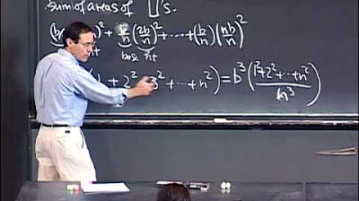
Lec 18 | MIT 18.01 Single Variable Calculus, Fall 2007

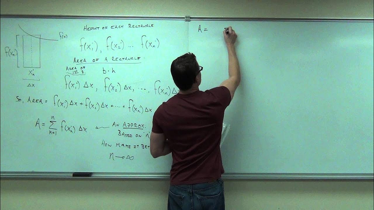
Calculus 1 Lecture 4.3: Area Under a Curve, Limit Approach, Riemann Sums

Calculus 1: Definition of the Integral Examples

Business Calculus - Math 1329 - Section 5.3 - The Definite Integral and Fundamental Thm of Calculus

Related Tags

Calculus Lessons Summation Notation Riemann Sums Definite Integrals Math Education Mr. Bean Area Approximation Infinite Series Math Concepts Educational Comedy