Tensor Calculus 7: Covector Field Components
TLDRThis educational video explores the concept of decomposing differential forms into their constituent components, building upon the fundamentals of tensor analysis. It demonstrates how differential forms, akin to vectors, can be expressed as linear combinations of basis differential forms, with coefficients derived from partial derivatives. The video uses concrete examples in Cartesian and polar coordinates to illustrate the process, highlighting the geometric interpretation of differential forms and their transformation rules, ultimately revealing the deep connection between differential forms and multivariable calculus.
Takeaways
- 📚 The video discusses breaking down differential forms into their components, building on the concept of tensor components and transformation rules.
- 🔗 It is recommended to watch previous videos on tensors for beginners before this one for better understanding.
- 📉 The differential operator 'd' is explained as taking a scalar field and producing a covector field by tracing level set curves and orienting them towards the positive scalar direction.
- ➕ The script highlights the linearity laws of differential forms, where addition and scaling of inputs or outputs yield the same result.
- 📍 The geometrical interpretation of the differential 'DF' is the directional derivative of a function 'f' with a velocity vector 'V' at a point.
- 📈 The video shows how differential forms can be expressed as linear combinations of special basis differential forms, with components determined by the number of lines pierced by vectors.
- 🔍 The script explains the action of covector fields on basis vectors, such as the partial derivatives with respect to 'x' and 'y', and their resulting directional derivatives.
- 🌐 The concept of dual basis for the space of all covectors is introduced, with epsilon 1 and epsilon 2 obeying special relationships that resemble the basis vectors.
- 📝 Any arbitrary covector can be written as a linear combination of epsilon 1 and epsilon 2, with the components representing the amount of lines pierced by each basis vector.
- 📚 The script provides a concrete example of expanding a covector field in Cartesian coordinates, using partial derivatives as scaling coefficients.
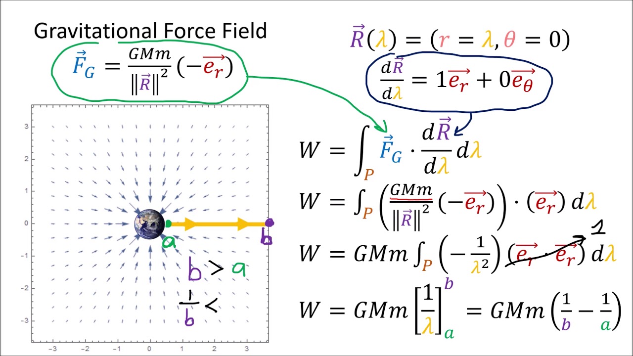
- 🌐 The video also covers the expansion of covector fields in polar coordinates, demonstrating the process with a scalar field and its corresponding covector field.
Q & A
What is the main topic of the video?
-The main topic of the video is breaking up differential forms into their components, which is an extension of the concepts covered in the 'Tensors for Beginners' series.
Why is it recommended to watch the 'Tensors for Beginners' videos before this one?
-It is recommended because the current video builds upon the concepts of covector components and transformation rules introduced in the 'Tensors for Beginners' series, providing a more advanced understanding.
What is the role of the del operator in the context of this video?
-The del operator is used to take a scalar field and produce a covector field by tracing out the level set curves of constant value and orienting the curves toward the positive scalar direction.
How do differential forms obey the linearity laws mentioned in the video?
-Differential forms obey linearity laws by allowing for the addition and scaling of inputs or outputs without changing the result, maintaining the same outcome in both cases.
Can you explain the geometrical interpretation of the directional derivative in the context of this video?
-The geometrical interpretation of the directional derivative is the rate of change of a function as it moves through a point with a velocity vector, which can be visualized as the function's slope in the direction of the velocity vector.
What is the significance of basis vectors in the context of differential forms?
-Basis vectors are significant because they allow us to write differential forms as linear combinations of special basis differential forms, which are scaled by components, providing a framework to understand and manipulate these forms.
How does the video explain the relationship between a scalar field and its corresponding covector field?
-The video explains that a scalar field's corresponding covector field can be obtained by considering the rate of change of the scalar field in the direction of basis vectors, which are represented by partial derivatives.
What is the Kronecker Delta and how does it relate to the covector fields discussed in the video?
-The Kronecker Delta is a function that equals 1 if its two indices are the same and 0 otherwise. It relates to covector fields by summarizing the relationship between epsilon covector fields and basis vectors, where epsilon I of EJ gives the Kronecker Delta IJ.
How does the video demonstrate the process of expanding a covector field as a linear combination of other covector fields?
-The video demonstrates this by using a concrete example of a scalar field and its covector field, showing how to calculate the coefficients for the linear combination using partial derivatives with respect to the basis vectors.
What is the purpose of using Einstein notation in the video?
-Einstein notation is used to compactly express the formulas for expanding covector fields into linear combinations of basis covector fields, simplifying the representation and making the relationships between components more clear.
How does the video connect the concepts of differential forms to those learned in multivariable calculus?
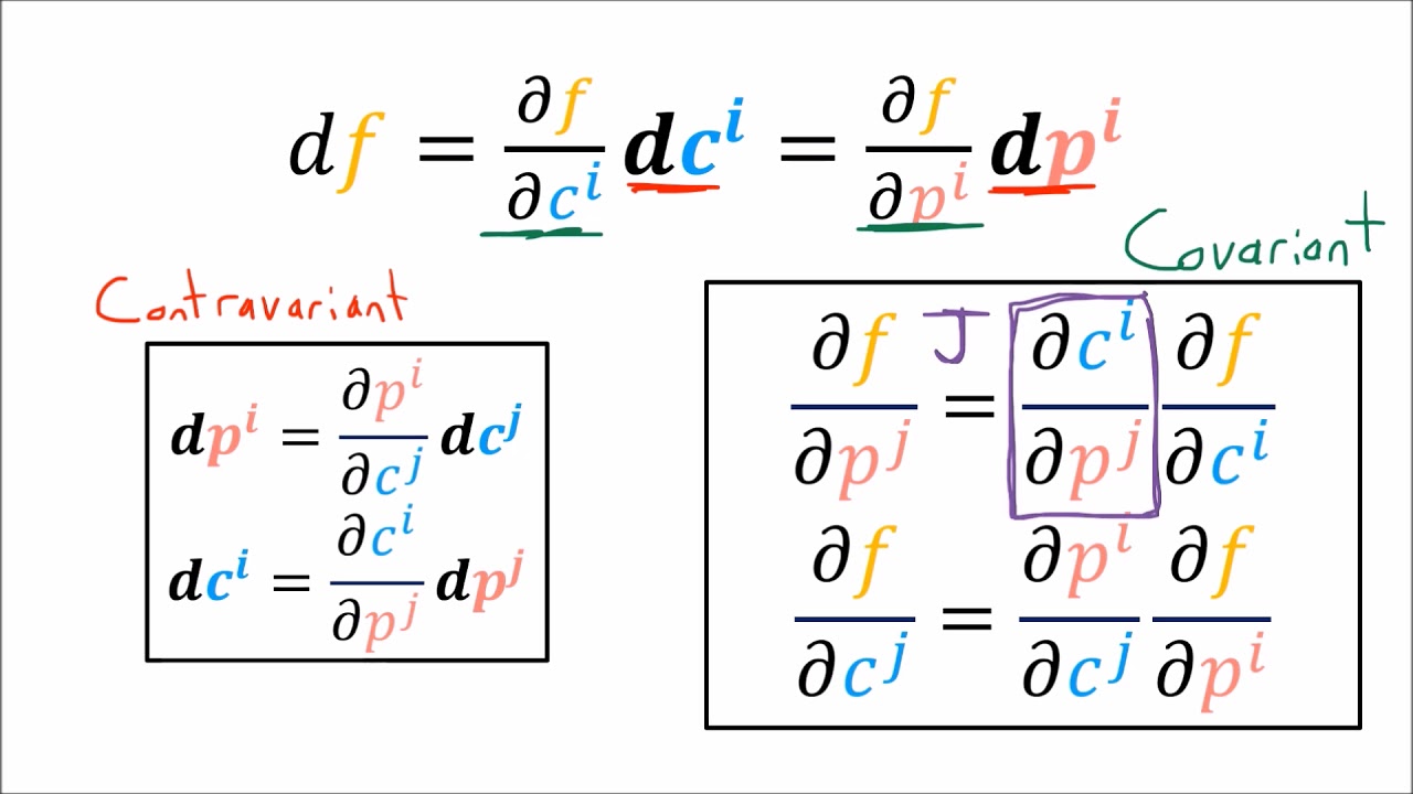
-The video connects these concepts by showing that the formulas used to expand differential forms are similar to those used for differentials in multivariable calculus, reinterpreting them as covector fields instead of just small changes in variables.
What will be the focus of the next video in the series?
-The next video will focus on the transformation rules for covector fields, explaining how basis covector fields are contravariant while covector field components are covariant.
Outlines
📚 Introduction to Differential Forms and Covector Fields
This paragraph introduces the concept of breaking down differential forms into their components, building upon the 'Tensors for Beginners' series. The video aims to show how differential forms can be expressed as linear combinations of special basis differential forms, similar to how vectors are represented in terms of basis vectors. It discusses the action of the differential operator 'd' on scalar fields to create covector fields and the linearity properties of these fields. The geometric interpretation of the directional derivative is also explained, setting the stage for the exploration of covector field components.
🔍 Decomposing Covector Fields into Basis Components
The second paragraph delves into the process of decomposing covector fields into their components by examining how different covector fields act on basis vectors, specifically the partial derivatives with respect to x and y. It explains how the covector fields DF, DX, and DY act on these basis vectors, resulting in partial derivatives. The paragraph establishes that DX and DY form a basis for all covector fields, analogous to how epsilon 1 and epsilon 2 serve as a basis for all covectors. The concept of using these basis fields to express any arbitrary covector field as a linear combination is introduced, with the components being determined by the number of lines pierced by the basis vectors.
📘 Applying Covector Field Expansion in Cartesian and Polar Coordinates
This paragraph demonstrates the application of covector field expansion through concrete examples in both Cartesian and polar coordinates. It shows how to calculate the coefficients for the linear combination of covector fields DX and DY by using partial derivatives. The example provided involves a scalar field F and its associated covector field DF, which is expanded using the calculated coefficients. The paragraph also discusses the geometric interpretation of these coefficients in the context of the covector field's orientation and spacing. The process is then extended to polar coordinates, showing the transformation of Cartesian coordinates to polar and the corresponding adjustments in the covector field expansion.
Mindmap
Keywords
💡Differential Forms
💡Covector Fields
💡Linearity Laws
💡Directional Derivative
💡Basis Vectors
💡Components
💡Kronecker Delta
💡Dual Basis
💡Einstein Notation
💡Polar Coordinates
💡Covariant and Contravariant
Highlights
The video explains the concept of breaking up differential forms into their components, building on the foundation of previous 'Tensors for Beginners' videos.
Introduction to differential forms and their geometrical interpretation as the directional derivative of a function with a velocity vector.
Differential forms obey linearity laws, allowing for the addition and scaling of inputs or outputs to yield the same result.
The method to compute the result of a covector field acting on a vector at a point by counting how many covector lines the vector pierces.
Differential forms can be written as linear combinations of special basis differential forms, similar to how vectors are represented.
Investigation of how different covector fields act on basis vectors, specifically the partial derivatives with respect to X and Y.
The directional derivative of a scalar field in the X and Y directions equates to the partial derivatives with respect to those variables.
The scalar field X results in a covector field where the DX basis vector pierces one line and the DY basis vector pierces none.
For the scalar field Y, the covector field DY has a component that changes with the value of Y, affecting the density of the covector field.
The importance of understanding the action of covector fields on basis vectors for breaking up covector fields into components.
The special covector epsilon 1 and epsilon 2 are introduced as the dual basis for the space of all covector fields.
Any arbitrary covector can be expressed as a linear combination of epsilon 1 and epsilon 2, with components indicating the number of lines pierced.
The process of determining the coefficients for the linear combination of covector fields DX and DY to represent a given covector field.
The demonstration that any covector field can be written as a linear combination of DX and DY using partial derivatives as scaling coefficients.
A concrete example of expanding a given scalar field's covector field as a linear combination of DX and DY, with calculated coefficients.
The geometric interpretation of the coefficients in the covector field, explaining the spacing and orientation of the field's curves.
The expansion of differential forms in polar coordinates, showcasing the process with a scalar field and its corresponding covector field.
The computation of partial derivatives in polar coordinates and their impact on the covector field's components.
The visual verification of the polar coordinate components of a covector field, ensuring they align with the expected orientation and spacing.
The generalization that differential forms can be expanded into linear combinations of basis covector fields, with components varying by the chosen basis.
The connection between the formulas for differential forms and the familiar differential formulas from multivariable calculus.
The预告 of the next video, which will cover the transformation rules for covector fields and the distinction between contravariant basis covector fields and covariant components.
Transcripts
Browse More Related Video


5.0 / 5 (0 votes)
Thanks for rating: