Converting a Higher Order ODE Into a System of First Order ODEs
TLDRThe video explains how to transform a higher-order linear, constant-coefficient differential equation into a system of first-order differential equations. Starting with a fourth-order equation, it demonstrates solving for the highest-order derivative and renaming all derivatives as new variables. This process leads to rewriting the equation in terms of first-order equations involving variables x1, x2, x3, x4. The script further illustrates converting the system into matrix form, showing how the original differential equation is represented as X' = AX, with X being the vector of functions and A the coefficient matrix. It also covers solving a second-order equation with initial conditions, emphasizing the transformation into vector form.
Takeaways
- 📚 The video explains the process of converting a higher-order linear constant-coefficient differential equation into a system of first-order differential equations.
- 🔍 The first step involves isolating the highest order derivative on one side of the equation to prepare for the transformation.
- 🔄 A renaming process is introduced where each derivative of the function, from the zeroth to the third, is assigned a new variable (x1, x2, x3, x4).
- 📉 The fourth derivative is recognized as equivalent to the first derivative of the third derivative, allowing for the substitution of variables.
- 📝 The original fourth-order differential equation is rewritten as a first-order equation in terms of the new variables, setting the stage for a system of equations.
- 🔑 The concept of a 'system' is introduced, showing how the differential equations for each new variable can be derived from the original equation.
- 📈 The system of differential equations is then written out explicitly, with each equation representing the derivative of a new variable.
- 📊 A matrix representation is used to simplify the system, showing how the system can be represented as a matrix equation X' = AX.
- 🌐 The video also covers a second-order differential equation with initial conditions, demonstrating how to handle non-homogeneous terms like cosine functions.
- 📌 Initial conditions are incorporated into the system, showing how to set up the initial state of the system using given values for the function and its derivative at a specific point.
- 🔍 The final form of the initial value problem is presented in vector form, highlighting the integration of the system of equations with the initial conditions.
Q & A
What is the main topic of the video?
-The main topic of the video is converting a higher-order linear constant-coefficient differential equation into a system of first-order differential equations.
What is the highest order of the differential equation discussed in the video?
-The highest order of the differential equation discussed in the video is fourth order.
What is the first step in converting a higher-order differential equation into a system of first-order equations?
-The first step is to solve for the highest order derivative and isolate it on one side of the equation.
How are the derivatives of the original variable renamed in the process?
-The derivatives are renamed as new variables, such as x1 for the zeroth derivative (X), x2 for the first derivative (X prime), x3 for the second derivative (X double prime), and x4 for the third derivative.
What is the significance of recognizing X_sub_4 as the third derivative in the process?
-Recognizing X_sub_4 as the third derivative allows us to express the fourth derivative as X_sub_four_prime, which helps in rewriting the original equation in terms of the new variables.
How does the video illustrate the transformation of the original equation into a system of first-order equations?
-The video illustrates this by substituting the new variables into the original equation and then observing that the derivatives of these new variables form a system of first-order equations.
What is the purpose of rewriting the original differential equation in terms of new variables?
-The purpose is to express the higher-order equation as a system of first-order equations, which is easier to solve and analyze, especially when using matrix representation.
How is the system of differential equations represented in matrix form?
-The system is represented in matrix form as X_prime = A * X, where X is the vector of the new variables and A is the matrix containing the coefficients of the derivatives.
What is an initial value problem in the context of differential equations?
-An initial value problem is a differential equation with specified initial conditions, which give the values of the function and its derivatives at a particular point in time.
How are initial conditions incorporated into the system of first-order differential equations?
-Initial conditions are incorporated by setting the values of the new variables at the initial time, which forms a constant vector C that represents the state of the system at time zero.
What is the role of the vector F in the matrix equation X_prime = A * X + F?
-The vector F represents the non-homogeneous part of the differential equation, which includes terms that are not dependent on the variables of the system, such as the cosine function in the given example.
Outlines
📚 Converting Higher-Order DEs to First-Order Systems
This paragraph introduces the process of transforming a fourth-order linear constant-coefficient differential equation into a system of first-order differential equations. The initial step involves isolating the highest order derivative on one side of the equation, which in this case is the fourth derivative. The equation is then rewritten with all terms involving derivatives of varying orders moved to the opposite side, effectively reducing their order. The next step is to rename each derivative of the original function, denoted as X, as new variables (x1 through x4), representing the function itself and its first, second, and third derivatives, respectively. The fourth derivative is then equated to the derivative of the third renamed variable (x4 prime). The paragraph concludes with the observation that the original fourth-order equation can now be expressed as a system of first-order equations in terms of these new variables.
🔍 Developing a System of Differential Equations from a Fourth-Order DE
The second paragraph delves deeper into the conversion process by illustrating how to derive a system of first-order differential equations from the fourth-order equation. It begins by defining the relationship between the renamed variables and their derivatives, such as x1 prime being equal to x2, and so on. This leads to the identification of three additional first-order differential equations involving the new variables x1, x2, x3, and x4. The paragraph then demonstrates how to represent these relationships in matrix form, with the left side of the matrix equation representing the vector of the variables' derivatives (X prime) and the right side being the product of a matrix (A) and the vector of the variables (X). The matrix A is constructed based on the coefficients of the derivatives in the original equation. The paragraph concludes with the representation of the system of equations in a compact matrix form, showcasing the transformation of the original higher-order differential equation into a manageable system of first-order equations.
📉 Incorporating Initial Conditions into a System of DEs
The final paragraph extends the discussion to include initial conditions in the system of differential equations derived from a second-order equation, which is an initial value problem. The process starts by isolating the highest derivative, in this case, the second derivative (x2 prime), and rearranging the terms to express it in terms of the original function and its first derivative. The variables are then renamed as before, with x1 representing the function and x2 representing its first derivative. The paragraph highlights the need to correct a mistake in the transcription of the equation and proceeds to establish the system of differential equations with the inclusion of a non-homogeneous term, cosine 3t. The system is then represented in vector and matrix form, with the addition of a forcing function vector. The initial conditions are carefully incorporated, with the initial values for x1 and x2 being specified. The paragraph concludes by presenting the entire initial value problem in vector form, emphasizing the transition from the original equation to a system of equations that can be solved with given initial conditions.
Mindmap
Keywords
💡Higher-order linear differential equation
💡Constant-coefficient
💡System of first-order differential equations
💡Derivative
💡Renaming variables
💡Matrix form
💡Initial value problem
💡Vector
💡Rewriting equations
💡Transformation
Highlights
Introduction to converting a higher-order linear, constant-coefficient differential equation into a system of first-order differential equations.
Starting with a fourth-order differential equation as the example to be converted.
First step: Solve for the highest order derivative and isolate it on one side of the equation.
Rewrite the equation with the highest order derivative on one side and the lower order derivatives on the other side.
Introduce new variables for each derivative of the original function: x1 for X, x2 for X', x3 for X'', and x4 for X'''.
Replace the original derivatives in the equation with the new variables.
Write the fourth derivative as x4', converting the original equation into a first-order equation in terms of the new variables.
Establish the relationships between the new variables and their derivatives, e.g., x2 = x1', x3 = x2', x4 = x3'.
Derive the system of first-order differential equations from these relationships.
Form the matrix equation X' = AX, where X is the vector of new variables and A is the coefficient matrix.
Convert a second-order differential equation with initial conditions into a similar system and matrix form.
Solve for the highest order derivative in the second-order equation, isolating it on one side.
Rename the variables and substitute them into the equation to form a system of first-order equations.
Express the system in matrix form with appropriate initial conditions.
Summarize the process of converting higher-order differential equations into systems of first-order differential equations and representing them in matrix form.
Transcripts
Browse More Related Video
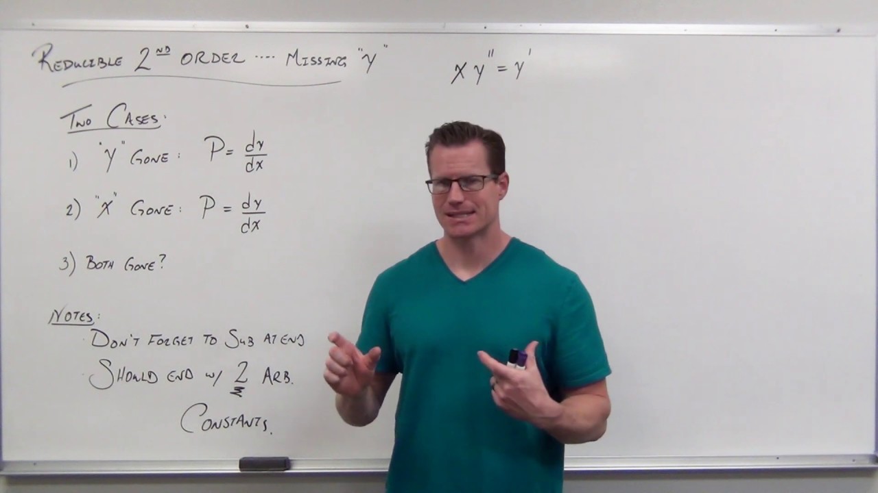
Reducible Second Order Differential Equations, Missing Y (Differential Equations 26)
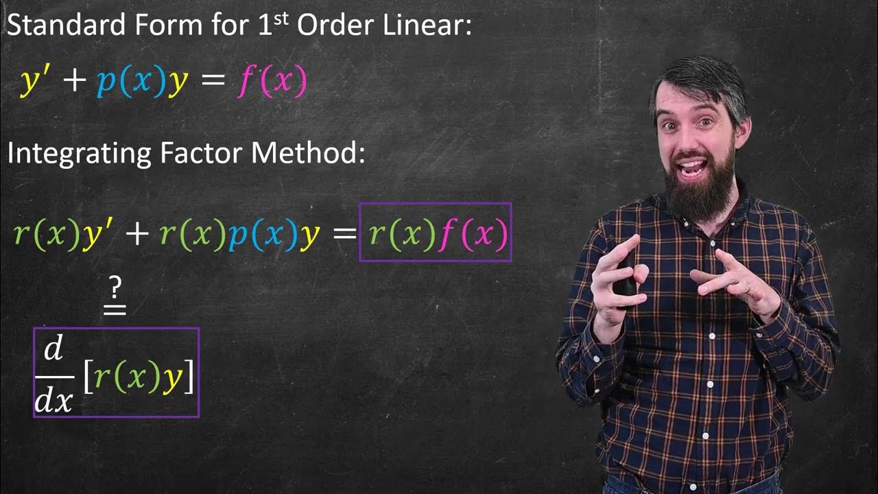
Linear Differential Equations & the Method of Integrating Factors

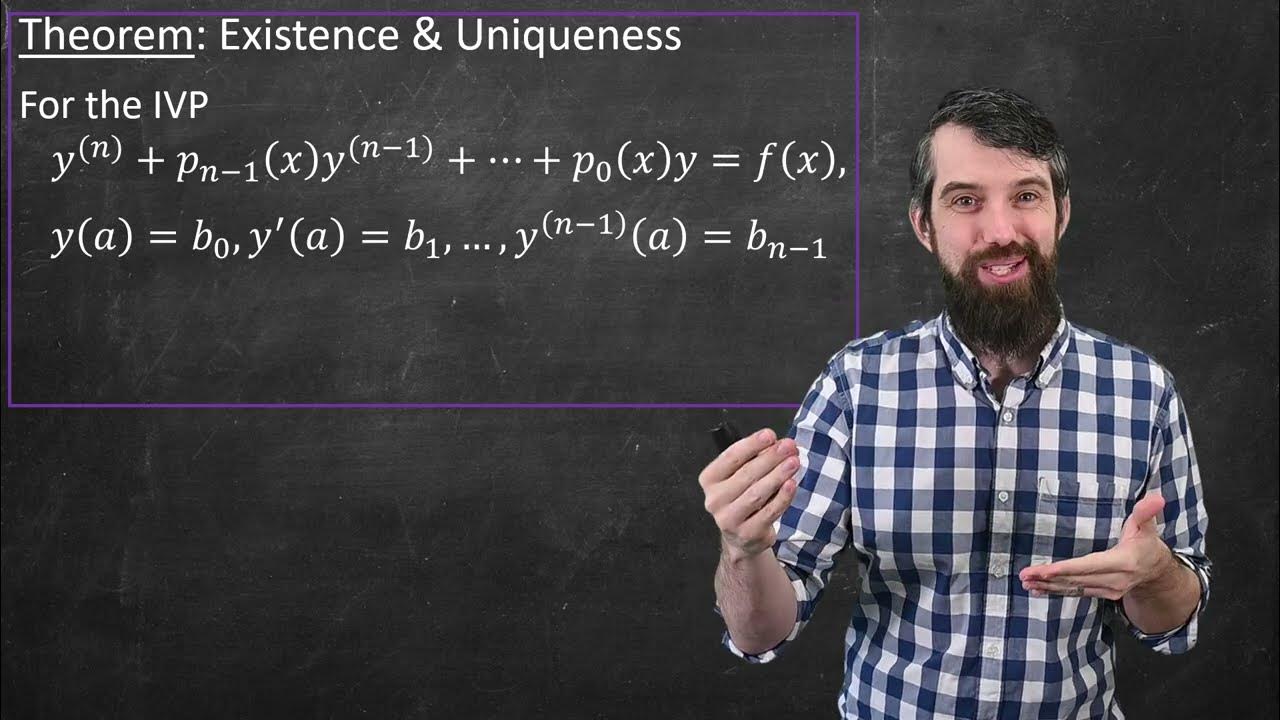
The Theory of 2nd Order ODEs // Existence & Uniqueness, Superposition, & Linear Independence
The Theory of Higher Order Differential Equations
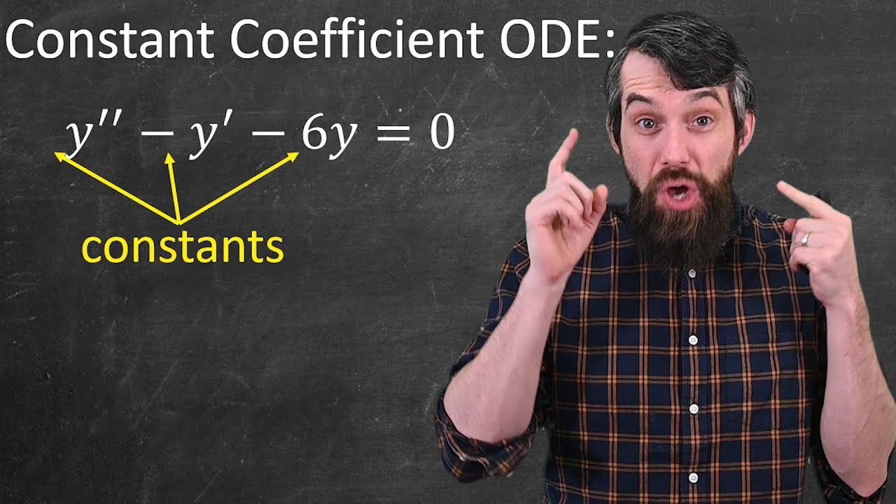
How to Solve Constant Coefficient Homogeneous Differential Equations
Differential Equations - Introduction - Part 1
5.0 / 5 (0 votes)
Thanks for rating: