2610 Chapter 8 Day 1

Brian Steffen

4 Mar 202437:09

EducationalLearning

32 Likes 10 Comments

TLDRThis educational video script delves into the concept of confidence intervals, using a population of heights as an example. It explains the process of calculating confidence intervals when the population mean and standard deviation are known, and when they are not. The script introduces the t-distribution for cases where the population standard deviation is unknown. It also discusses the impact of sample size on the width of confidence intervals and the importance of proper random sampling in statistical inference. The instructor guides viewers through practical examples, including using online applets for visualizing the sampling distribution and understanding the relationship between confidence levels and interval width.

Takeaways

📚 The lesson focuses on understanding 'Confidence Intervals' as presented in Chapter 8 of the textbook.
🧍 The initial data collected on people's heights is considered the population for this exercise, with 71 data points.
🎯 The population mean (mu) is assumed to be the average height, and the population standard deviation (Sigma) is symbolized by the Greek letter sigma.
📉 The assumption of normal distribution for the population height is made to simplify calculations.
🤵 The probability of a randomly selected individual being over 72 inches tall is calculated using the Z-score method.
🔢 The Z-score formula is z = (x - mu) / Sigma, which is applied with the given population mean and standard deviation.
📊 The use of online applets for determining probabilities associated with Z-scores is demonstrated.
👥 When considering a random group of five, the sampling distribution of their average height is also assumed to be normal, due to the normality of the parent population.
📐 The standard deviation of the sampling distribution (X-bar) is calculated as Sigma divided by the square root of the sample size (n).
🔄 The empirical rule and the concept of a confidence interval are introduced for estimating the population mean when the true mean is unknown.
📝 The construction of a confidence interval involves using the sample mean (x-bar), the Z-score for the desired confidence level, and the standard error (Sigma/√n).
📉 The students are tasked with using online tools to explore how changes in confidence level affect the width of the confidence interval.
📚 The importance of correctly interpreting a confidence interval is emphasized, avoiding the incorrect notion that there's a certain probability the true mean falls within the interval.
📈 The effect of increasing the sample size on the confidence interval's width and the precision of the estimate is discussed.
📊 The transition from using the Z-distribution to the T-distribution when the population standard deviation is unknown is explained, introducing the concept of degrees of freedom.

Q & A

What is the main topic of Chapter 8 in the textbook?
-The main topic of Chapter 8 is confidence intervals.
What is the difference between x̄ and μ in the context of this script?
-In the context of this script, x̄ (x-bar) represents the sample mean, while μ (mu) is the population mean.
What is assumed about the population height distribution in this script?
-It is assumed that the population height distribution is normal, which allows for the use of z-scores and normal distribution properties.
How is the probability of a randomly selected person being over 72 inches tall calculated?
-The probability is calculated by finding the z-score for 72 inches, which is (72 - μ) / σ, and then using a standard normal distribution table or applet to find the corresponding area.
What is the standard deviation of the sampling distribution if the population standard deviation is 45.172 and the sample size is 5?
-The standard deviation of the sampling distribution, also known as the standard error, is the population standard deviation divided by the square root of the sample size, so it would be 45.172 / √5.
What is the difference between a confidence interval for an individual value and a confidence interval for a sample mean?
-A confidence interval for an individual value predicts the range within which a single value is likely to fall, while a confidence interval for a sample mean estimates the range within which the population mean is likely to be, based on the sample mean.
What is the empirical rule, and how does it relate to the construction of confidence intervals?
-The empirical rule states that for a normal distribution, approximately 95% of the data falls within two standard deviations of the mean. In the context of confidence intervals, it suggests that if the process of selecting samples is repeated many times, about 95% of the sample means will fall within two standard errors of the population mean.
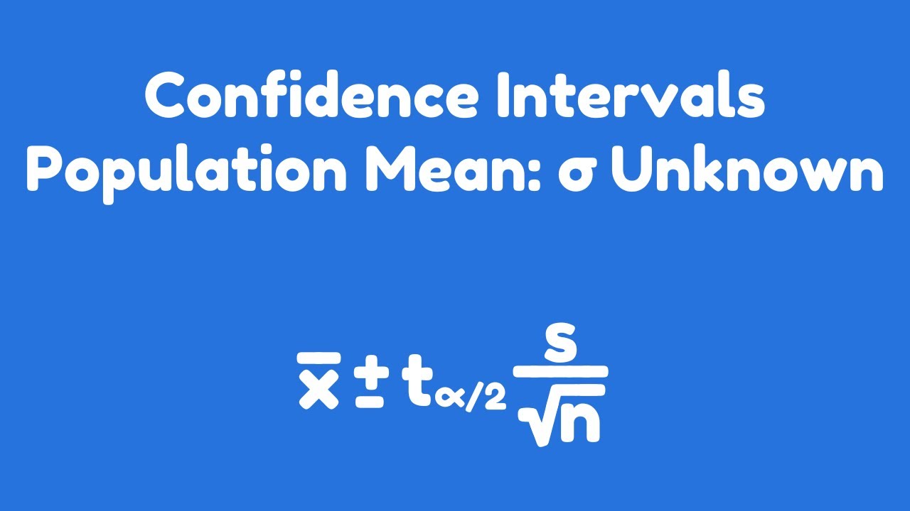
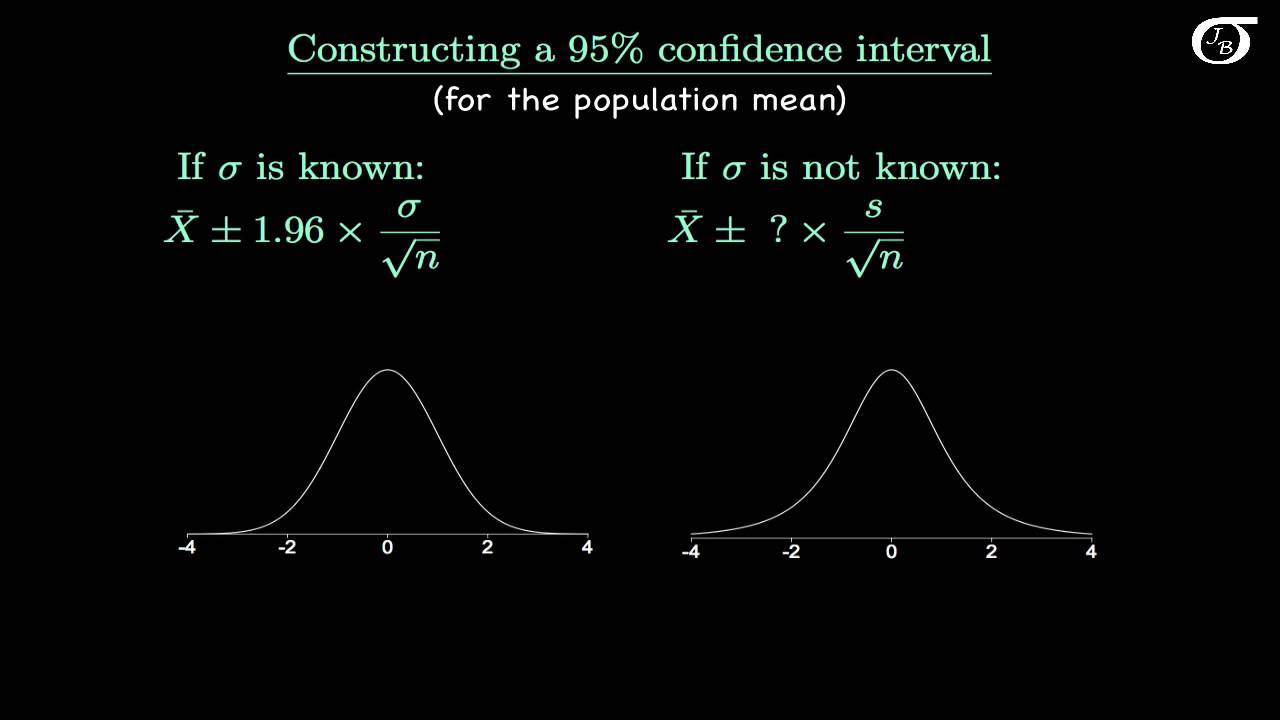
What is the formula for calculating a confidence interval for a population mean when the population standard deviation is known?
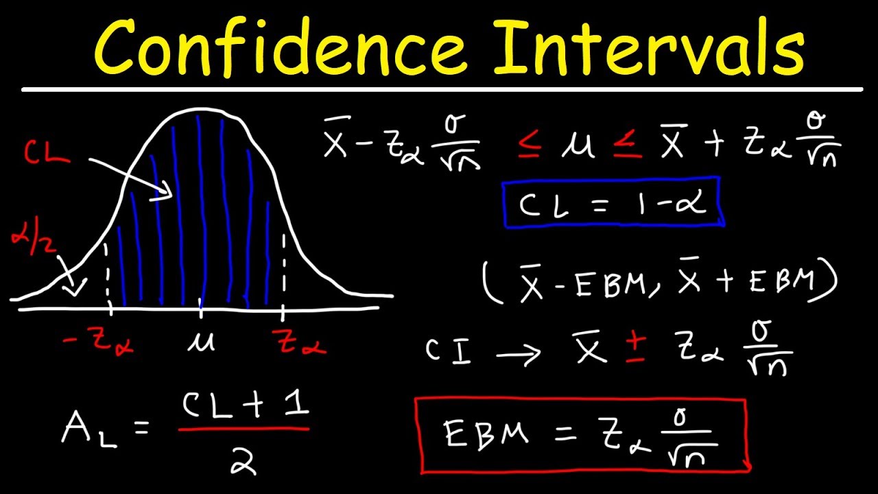
-The formula for calculating a confidence interval is x̄ ± Z * (σ / √n), where x̄ is the sample mean, Z is the z-score corresponding to the desired confidence level, σ is the population standard deviation, and n is the sample size.
What is the relationship between the confidence level and the margin of error in a confidence interval?
-The confidence level represents the percentage of intervals that would contain the population parameter if the sampling process were repeated many times. The margin of error is the amount added and subtracted from the sample statistic to create the confidence interval. A higher confidence level results in a larger margin of error to ensure the desired level of confidence.
What is the purpose of the students' t-distribution in constructing confidence intervals when the population standard deviation is unknown?
-The students' t-distribution is used instead of the z-distribution when the population standard deviation is unknown. It accounts for the additional uncertainty due to estimating the standard deviation from the sample, resulting in a distribution with thicker tails, which leads to a wider confidence interval.
How does the sample size affect the width of a confidence interval?
-As the sample size increases, the standard error (σ / √n) decreases, which makes the confidence interval narrower. Conversely, a smaller sample size results in a larger standard error and a wider confidence interval.

Outlines

00:00

📚 Introduction to Confidence Intervals

The script begins with an introduction to Chapter 8, focusing on the concept of confidence intervals. It explains the shift from considering sample data to a hypothetical population of heights. The population mean (mu) and standard deviation (Sigma) are identified, and the assumption of a normal distribution is made. The script then explores the probability of an individual's height being over 72 inches using the z-score formula and a normal distribution curve. The calculation process and the resulting probability of 27.86% are detailed.

05:01

👥 Sampling Distribution of Means

This paragraph delves into the concept of the sampling distribution of means, emphasizing that if the population distribution is normal, the sampling distribution of averages will also be normal. It discusses the standard deviation of the sampling distribution and how it relates to the original population standard deviation, divided by the square root of the sample size (n). The script then calculates the probability of a random group of five people having an average height over 72 inches, using the sampling distribution and arriving at a 99.46% chance.

10:02

🔍 Estimating the Population Mean

The script discusses the limitations of a single point estimate and introduces the method of creating a confidence interval to estimate the population mean more accurately. It explains the empirical rule and how it applies to the sampling distribution being normal. The process of constructing a 95% confidence interval is demonstrated, using the sample mean, standard deviation, and the Z-score for the desired confidence level. The resulting interval and its interpretation are provided.

15:04

📉 Understanding Confidence Intervals and Margin of Error

This section clarifies the terms used in constructing confidence intervals, such as margin of error, standard error, and confidence level. It explains the relationship between these terms and how they contribute to the interval estimate. The script also corrects common misconceptions about interpreting confidence intervals, emphasizing that the interval either contains the true mean or it does not, rather than having a probability of containing it.

20:05

📈 Visualizing Confidence Intervals with Sample Size Variation

The script uses an online applet to visually demonstrate the effect of sample size on the width of confidence intervals. It shows that as sample size increases, the standard deviation of the sampling distribution decreases, leading to narrower intervals. The empirical rule is again mentioned, illustrating that larger sample sizes result in more confidence intervals containing the true mean.

25:05

🤔 Dealing with Unknown Population Standard Deviation

This part addresses the scenario where the population standard deviation is unknown and must be estimated using the sample standard deviation (s). It introduces the student's t-distribution as the appropriate distribution to use in place of the Z-distribution when the population standard deviation is unknown. The script explains the concept of degrees of freedom and how they relate to the shape of the t-distribution.

30:07

📝 Calculating Confidence Intervals with the T-Distribution

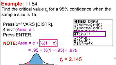
The script provides a step-by-step guide on calculating a confidence interval when the population standard deviation is unknown, using the t-distribution. It demonstrates finding the t-value from a t-table based on the degrees of freedom and the desired confidence level. The calculation of the margin of error and the final confidence interval is shown, along with the correct way to interpret the results.

35:09

📉 Comparing Confidence Intervals and Assignment Tasks

The final paragraph wraps up the video script by summarizing the process of creating confidence intervals and setting an assignment for students. It asks students to compare two 95% confidence intervals created in the script, identify which is wider, and explain why. The script also directs students to complete online applets for further practice and to submit their findings via email for participation points.

Mindmap

Keywords

💡Confidence Interval

A confidence interval is a range of values, derived from a statistical model, that is likely to contain the value of an unknown population parameter. In the video, the concept is central to understanding how to estimate the mean height of a population based on a sample. For example, the instructor calculates a 95% confidence interval for the mean height of a group, indicating that they are 95% confident the true mean lies within a certain range.

💡Population Mean (Mu, μ)

The population mean, often denoted by the Greek letter mu (μ), is the average of a population's data. In the script, the instructor initially assumes the known population mean to demonstrate calculations. Later, when the population mean is unknown, the sample mean is used as an estimate, showcasing the transition from known to unknown parameters in statistical analysis.

💡Sample Mean (x-bar)

The sample mean, represented as x-bar (x̄), is the average of the values in a sample used to estimate the population mean. The video script discusses how x-bar is used when the true population mean is unknown, and it is calculated from the heights of individuals in the sample to make inferences about the entire population.

💡Standard Deviation (Sigma, σ)

The standard deviation, symbolized by sigma (σ), measures the amount of variation or dispersion in a set of values. In the video, sigma is initially the standard deviation of the population, which is later replaced by the sample standard deviation when the population standard deviation is unknown.

💡Normal Distribution

A normal distribution, also known as a Gaussian distribution, is a probability distribution that is symmetrical and defined by its mean and standard deviation. The instructor assumes the population height follows a normal distribution, which allows for the use of z-scores and the properties of the normal curve to calculate probabilities and confidence intervals.

💡Z-Score

A z-score represents the number of standard deviations an element is from the mean in a normal distribution. The video uses z-scores to calculate the probability of an individual's height being over a certain value, demonstrating the application of z-scores in statistical inference.

💡Sampling Distribution

A sampling distribution is the probability distribution of a given statistic based on a random sample. The script explains that if the population distribution is normal, the sampling distribution of the sample mean (X-bar) is also normal, which is crucial for understanding how confidence intervals are constructed.

💡Central Limit Theorem

The central limit theorem states that the distribution of sample means approximates a normal distribution as the sample size gets larger, regardless of the population's distribution. While the video script mentions this theorem, it emphasizes that the normality of the sampling distribution in the example is due to the normality of the population, not the theorem.

💡Margin of Error

The margin of error is the range plus or minus a certain value that indicates the potential difference between the true population value and the sample statistic. In the video, the margin of error is calculated as part of the confidence interval and is used to express the precision of the estimate.

💡Students T-Distribution

The Student's t-distribution is a type of probability distribution used when the sample size is small and the population standard deviation is unknown. The video script introduces the t-distribution as an alternative to the z-distribution for constructing confidence intervals when estimating the population mean with a sample standard deviation.

💡Degrees of Freedom (DF)

Degrees of freedom represent the number of independent values in a set that can vary without restriction. In the context of the video, the degrees of freedom for the t-distribution is the sample size minus one, which determines the shape of the t-distribution and is used to find the critical t-value for a given confidence level.

Highlights

Introduction to Chapter 8 on Confidence Intervals.

Population of heights considered with 71 data points.

Mu as the population average and Sigma as the population standard deviation.

Assumption of normal distribution for population height.

Calculation of probability for a randomly selected person's height over 72 inches using z-scores.

Use of online applets for determining areas under the normal curve.

Interpretation of the probability result for an individual's height.

Transition to sampling distribution for a group of five people's average height.

Explanation of the central limit theorem and its relation to sampling distributions.

Calculation of the standard deviation of the sampling distribution.

Determination of the probability for a group's average height being over 72 inches.

Demonstration of constructing a confidence interval using sample data.

Difference between point estimate and interval estimate explained.

Use of the empirical rule and Z-values for constructing confidence intervals.

Interpretation of the confidence interval and its meaning.

Adjustment of confidence intervals when the population standard deviation is unknown.

Introduction to the Student's T-distribution for cases without known Sigma.

Explanation of degrees of freedom and their impact on the T-distribution.

Demonstration of calculating a confidence interval using the T-distribution.

Assignment for students to compare two confidence intervals and explain which is wider.

Encouragement for students to engage with textbook resources and complete practice problems.

Transcripts

Browse More Related Video

Confidence Intervals | Population Mean: σ Unknown

Confidence Interval Concept Explained | Statistics Tutorial #7 | MarinStatsLectures

Elementary Statistics - Chapter 7 - Estimating Parameters and Determining Sample Sizes Part 2

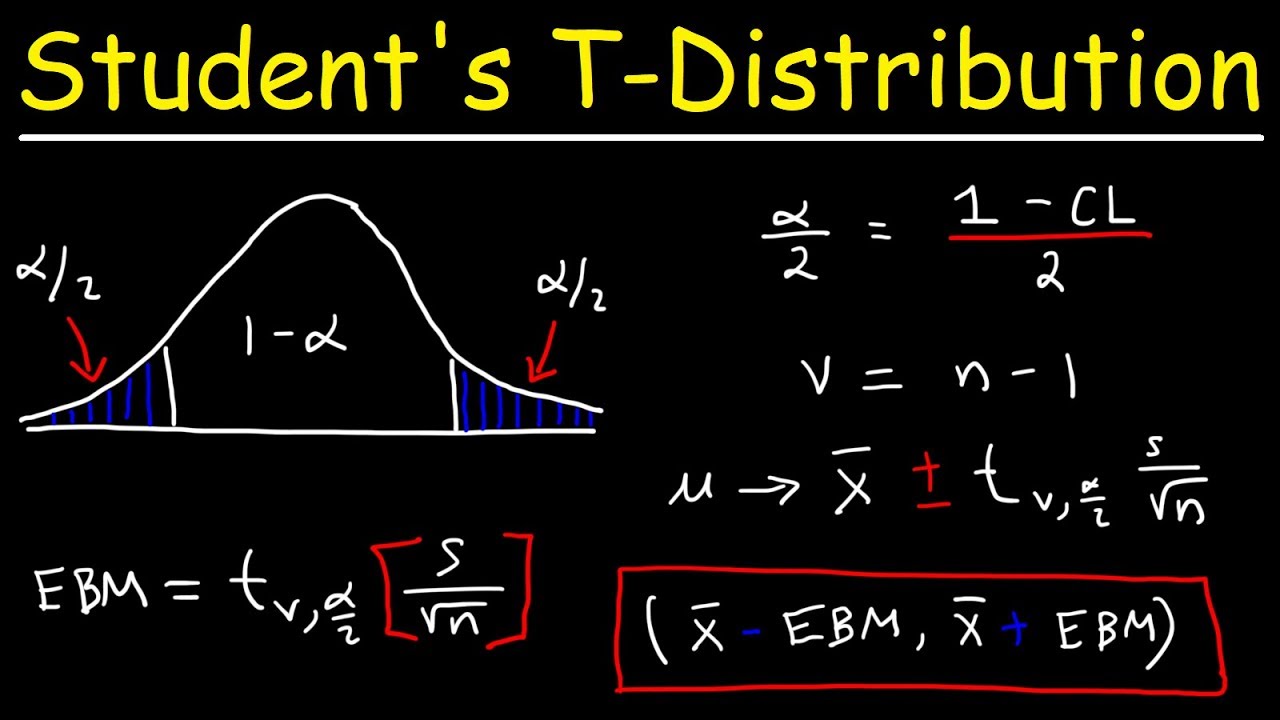
Student's T Distribution - Confidence Intervals & Margin of Error

Introduction to the t Distribution (non-technical)

How To Find The Z Score, Confidence Interval, and Margin of Error for a Population Mean

Related Tags

Confidence Intervals Statistics Normal Distribution Sampling Distribution Z-Score T-Distribution Population Mean Sample Size Standard Deviation Statistical Analysis Educational Tutorial