Calculus AB Lesson 7.3: Area Between Curves
TLDRThis lesson teaches how to calculate the area between two curves using definite integrals, a fundamental concept in calculus. The instructor explains how to set up Riemann sums with both vertical and horizontal rectangles, emphasizing the importance of identifying the correct top and bottom functions for each slice. The script covers various examples, including scenarios where the curves intersect or do not pass the vertical line test, requiring piecewise functions. The process involves finding points of intersection, setting up integral expressions, and evaluating them to find the exact area between the curves.
Takeaways
- 📚 The lesson focuses on calculating the area between two curves using definite integrals, which is an extension of the concept of Riemann sums.
- 📏 To find the area of a rectangle in the context of Riemann sums, one must multiply the width (Δx) by the height (difference in y-values of the curves).
- 🔍 Identifying the points of intersection of the two curves is crucial as they determine the limits of integration for the definite integral.
- 📐 The width of each rectangle in the Riemann sum is represented by Δx, and the height is given by the difference between the functions f(x) and g(x) at a given x.
- 📈 The definite integral that represents the exact area between the curves is written as the integral from 'a' to 'b' of [f(x) - g(x)] dx, where 'a' and 'b' are the x-values of the points of intersection.
- 🧩 The process involves breaking down the area between the curves into smaller rectangles and summing their areas, which is analogous to the Riemann sum approach.
- 🔢 The area between the curves can be found by subtracting the integral of the lower function from the integral of the upper function over the given interval.
- 🤔 The choice between using vertical or horizontal 'slices' (rectangles) for setting up the integral depends on the orientation that avoids the top and bottom of the rectangle touching the same function, simplifying calculations.
- 📉 When functions do not pass the vertical line test, indicating they are not functions but rather graphs, horizontal rectangles may be more appropriate for the Riemann sum.
- ✂️ For certain problems, it may be necessary to split the area into multiple regions and calculate the integral for each region separately, especially when the functions change their relative positions.
- 📝 The script also covers examples where the area calculation requires solving equations to find the x-values corresponding to the y-values at the limits of integration, emphasizing the importance of correctly setting up the integral.
Q & A
What is the main topic of this lesson?
-The main topic of this lesson is learning how to find the area between two curves using definite integrals.
What is the purpose of finding the width and height of a rectangle in the context of this lesson?
-The width and height of a rectangle are used to calculate the area of each rectangle in a Riemann sum, which approximates the area under a curve. This is essential for understanding how to find the area between two curves.
How is the width of each rectangle in the Riemann sum determined?
-The width of each rectangle is determined by the horizontal distance across the base, which is found by subtracting the left x-value from the right x-value (Δx = x_k - x_(k-1)).
What is the general expression for the height of a rectangle in the Riemann sum?
-The height of each rectangle is given by the vertical distance, which is the difference between the top y-value (f(x_k)) and the bottom y-value (g(x_k)) of the rectangle.
How do you calculate the area of each rectangle in the Riemann sum?
-The area of each rectangle is calculated by multiplying the base (width, Δx) by the height (f(x_k) - g(x_k)).
What is the Riemann sum and how does it relate to definite integrals?
-The Riemann sum is a method of approximating the definite integral (area under a curve) by summing the areas of rectangles. As the number of rectangles approaches infinity, the Riemann sum converges to the exact value of the definite integral.
How do you find the points of intersection of two curves to determine the interval for integration?
-You find the points of intersection by setting the equations of the two curves equal to each other and solving for x, which gives you the endpoints of the interval for integration.
What is the general expression for the definite integral that represents the area between two curves?
-The general expression for the definite integral representing the area between two curves is ∫(a to b) [f(x) - g(x)] dx, where f(x) is the top function, g(x) is the bottom function, and 'a' and 'b' are the x-values of the points of intersection.
Why might it be challenging to set up an integral to find the area between two curves if the curves are not functions?
-It might be challenging because if the curves are not functions (fail the vertical line test), you may need to use piecewise-defined functions, which can complicate the setup of the integral.
What is the difference between using vertical and horizontal rectangles (slices) in setting up the integral for the area between curves?
-Vertical rectangles use the difference in y-values (top minus bottom) and horizontal distances (right x minus left x), while horizontal rectangles use the difference in x-values (right function - left function) and vertical distances (top y minus bottom y). The choice between vertical and horizontal rectangles depends on the specific problem and which setup is simpler.
How can you determine whether to use a vertical or horizontal slice for finding the area between curves?
-You can determine the easier method by visually inspecting the curves and checking whether the top and bottom functions remain consistent when drawing rectangles. If the functions change or the same function touches both the top and bottom of the rectangle, a different method or a piecewise approach may be necessary.
Outlines
📚 Introduction to Finding Area Between Curves
This paragraph introduces the concept of calculating the area between two curves using definite integrals, reminiscent of Riemann sums. The focus is on understanding the width and height of rectangles that approximate the area under a curve, and the importance of identifying the right and left x-values for the width of these rectangles. The paragraph guides the learner to consider the vertical distance between the curves as the height of the rectangles and sets the stage for the development of the integral expression for the area.
📐 Calculating Rectangle Dimensions in Definite Integrals
The second paragraph delves deeper into the specifics of calculating the dimensions of rectangles used in approximating areas under curves. It explains how to find the width of each rectangle as ΔX, the change in X, and the height as the difference in Y values between two functions, f(X) and g(X). The area of each rectangle is then expressed as the product of its base (ΔX) and height [f(X_k) - g(X_k)]. The paragraph also encourages the learner to consider the sum of areas of all rectangles to approximate the total area between the curves.
🧩 Summation of Rectangle Areas and Transition to Definite Integrals
Building upon the previous discussion, this paragraph introduces the summation of the areas of all rectangles to find the total area between two curves. It presents the transition from a Riemann sum to a definite integral, both conceptually and notationally, to represent the exact area. The paragraph explains the use of limits to approach infinity for the number of rectangles and introduces the integral notation with its lower and upper bounds to encapsulate the area between the curves.
🔍 Intersection Points and Setting Up Definite Integrals
The focus shifts to practical application as the paragraph discusses finding the area between two given functions by first determining their points of intersection, which define the interval for the definite integral. It illustrates the process of setting up integral expressions for the area between the curves by considering the top and bottom functions, f(X) and g(X), and emphasizes the importance of finding where the curves intersect to establish the correct limits for integration.
📉 Understanding the Concept of Top and Bottom Functions in Area Calculation
This paragraph explores the concept of top and bottom functions in the context of calculating areas between curves. It explains that the area is found by integrating the difference of the top function minus the bottom function over the interval defined by the points of intersection. The paragraph also discusses the importance of recognizing which function is above the other within the interval and how this affects the setup of the integral.
🤔 Reflecting on the Methodology of Area Calculation Between Curves
The paragraph encourages reflection on the methodology used for calculating areas between curves. It highlights the flexibility of the method, which can accommodate functions that are below the x-axis or intersect in various ways. The discussion emphasizes understanding the significance of vertical distances (top minus bottom) and horizontal distances (right minus left) in setting up integrals for areas, whether using vertical or horizontal rectangles.
📝 Detailed Steps for Calculating Areas with Piecewise Functions
This paragraph provides a detailed walkthrough of calculating areas between curves when the curves are not functions, requiring piecewise definitions. It discusses the challenges of using vertical rectangles in such cases and suggests using horizontal rectangles instead. The explanation includes how to adjust the notation and setup for horizontal rectangles, including identifying the width (ΔY) and height (right X minus left X) of the rectangles and setting up the integral with the correct limits and differential (dy).
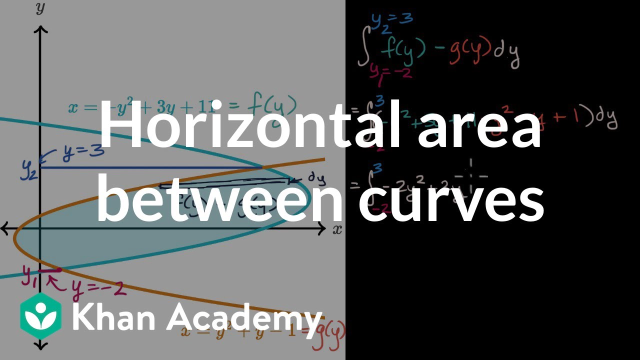
🔢 Examples of Setting Up Integrals for Areas with Horizontal Rectangles
The paragraph presents examples of setting up integrals for areas between curves using horizontal rectangles. It demonstrates how to identify the right and left X values as functions of Y, how to determine the correct interval for integration based on Y values, and how to express the area as the integral of the difference between the right and left X functions with respect to Y (dy). The examples illustrate the process of solving for X and setting up the integral correctly.
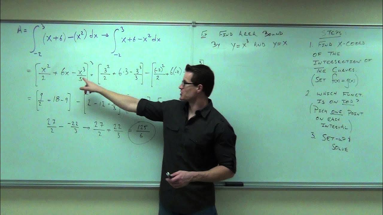
🏞️ Visualizing and Calculating Areas with Multiple Regions
This paragraph extends the concept to calculate areas in regions bounded by multiple curves and axes. It describes the process of dividing the region into subregions, each requiring separate integrals due to different functions being on top or bottom within each subregion. The explanation includes identifying the correct functions for each subregion, setting up the integrals with appropriate limits, and adding the results to find the total area.
🤷♂️ Challenges in Choosing Between Vertical and Horizontal Slices
The final paragraph discusses the critical thinking required to decide whether to use vertical or horizontal slices for calculating areas between curves. It highlights situations where one method may be more straightforward than the other, such as when the same function touches both the top and bottom of a rectangle in the chosen orientation. The paragraph encourages the learner to consider the ease of setting up the integral and the clarity of the function relationships when making this choice.
Mindmap
Keywords
💡Definite Integral
💡Riemann Sums
💡Width of Rectangles
💡Height of Rectangles
💡Area of Rectangles
💡Top Function
💡Bottom Function
💡Intersection Points
💡Vertical Line Test
💡Piecewise-Defined Function
Highlights
Introduction to calculating the area between two curves using definite integrals.
Understanding the concept of Riemann sums in relation to finding areas under curves.
Deriving expressions for the width and height of rectangles in a Riemann sum.
Generalizing the width of rectangles as ΔX in definite integral notation.
Calculating the height of rectangles using the difference between two function values.
Formulating the area of each rectangle in a definite integral context.
Summing the areas of all rectangles to approximate the area between curves.
Transitioning from Riemann sums to definite integrals for exact area calculation.
Setting up definite integrals to find the area between curves with given functions.
Finding intersection points of curves to determine the limits of integration.
Graphical and algebraic methods to find points of intersection for integral setup.
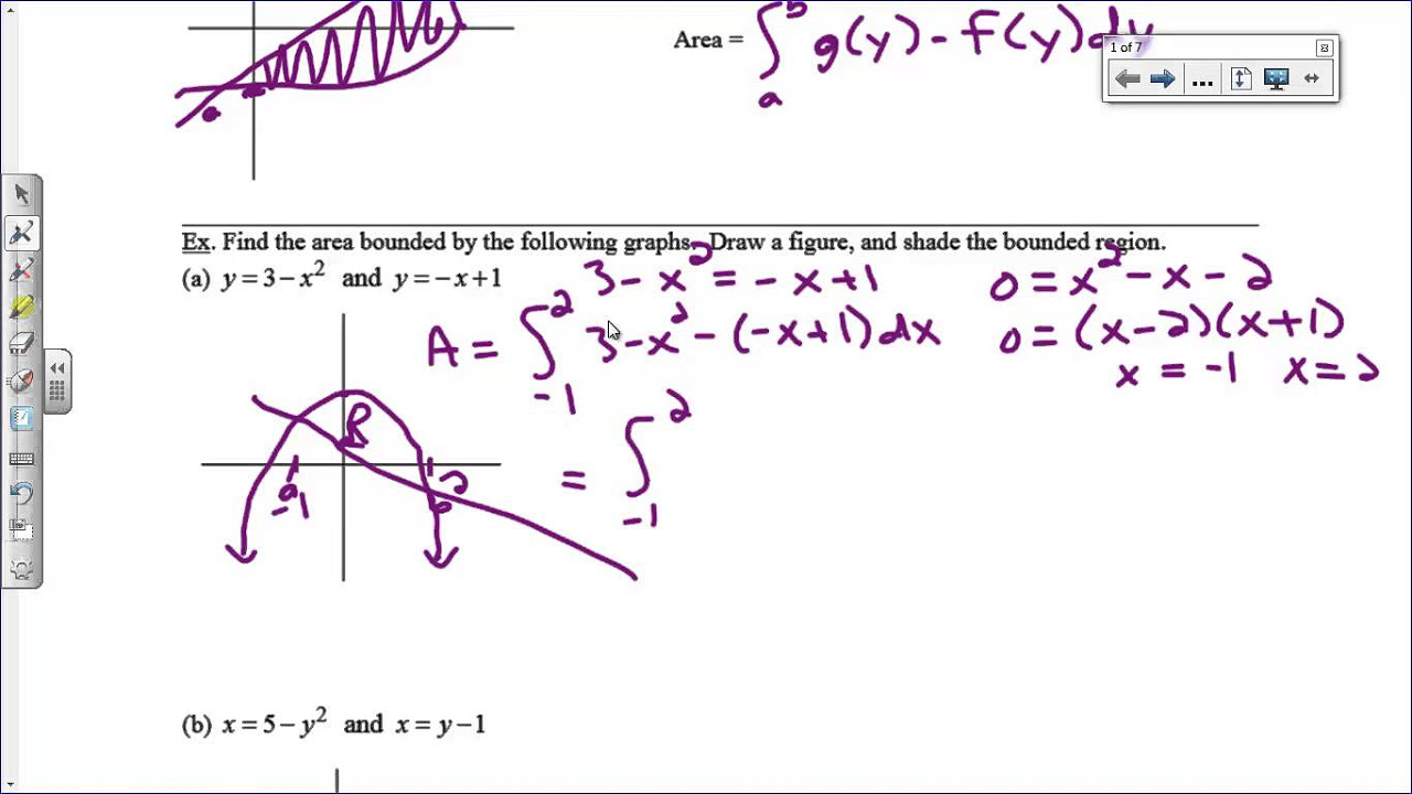
Writing integral expressions for the area between a quadratic and a linear function.
Subtracting integrals to find the area between two functions on a given interval.
Dealing with functions that do not pass the vertical line test and require piecewise definitions.
Using horizontal rectangles instead of vertical for certain integrals.
Setting up integrals with horizontal rectangles and dy instead of dx.
Solving equations for x to find the right and left x-values in horizontal integrals.
Examples of finding areas with horizontal and vertical slices and choosing the easier setup.
Critical thinking about when to use vertical vs. horizontal slices for area calculation.
Transcripts
Browse More Related Video

Calculus AB Homework 7.3 Area Between Curves
Area of a Region Between Two Curves
Calculus 1 Lecture 5.1: Finding Area Between Two Curves
Horizontal area between curves | Applications of definite integrals | AP Calculus AB | Khan Academy

Area Between Two Curves

Washer method rotating around vertical line (not y-axis), part 1 | AP Calculus AB | Khan Academy
5.0 / 5 (0 votes)
Thanks for rating: